Basically every machine learning AI problem is now solved using deep learning. Deep learning is the approach of using neural networks to learn from data, in this approach we don’t need to decide on what the model (neural network) should do, we just need to give it the data and the model will learn to do the task.

At its core, deep learning relies on lots of data and the concept of high dimensional features (more below). This is a first blog post covering the fundamental building blocks of deep learning.

Learning from Data

All of AL and ML uses lots and lots of data. Without it you can’t really get anywhere. So what actually happens when we learn from data? Well, what we want is to learn a model (Neural Network) that can map inputs to outputs. A great example is the MNIST dataset, which is a dataset of handwritten digits. We want to learn a model that can map an image of a handwritten digit to the correct digit. To do this, we create a model and then repeatedly show the data to the model, given that we know the correct answers (the digit). We can then adjust the model based on the data it got wrong.

This process is known as training the model. Where we evaluate how corret the model is using a loss function, and then adjust the model by changing the parameters (millions of numbers that describe the model) based on the loss function. We know how to change the parameters by taking the gradient of the loss function, this tells us how to change the parameters to get a better model.

This will all make sense soon, I promise.

Fundamentals of Deep Learning

Vectors

AI is based on high dimensions, and what I mean by this is having many ways that you can change a number to get many combinations. If we look at a single number we can only change it in one way, but if we look at a vector we can change it in many ways.

Looking at the first vector we can change $x_1$ and $x_2$ to get many combinations. But if we look at the second vector we can change $x_1$, $x_2$ and $x_3$ to get even more combinations of $\mathbf{x}$. This is exactly why we use vectors in deep learning, we can create many vectors that represent the complexities and nuances of the data, such as images of numbers.

Features

If you are interested in computer vision you will have heard the term features a lot. Confusingly features can mean two things: 1. the actualy parts of the image that make something a class (e.g. the face of the cat) and 2. the vectors that the model learns to extract from the data. It’s always good to clarify what someone means by features, do they mean in the data or in the model?

Neural Networks

A neural network consists of many layers which each transform the data in some way. The fundamental building block is the fully connected layer, mathematically represented as:

\(\mathbf{y} = \sigma(\mathbf{W} \mathbf{x} + \mathbf{b})\) where:

$\mathbf{x}$ is the input vector,
$\mathbf{W}$ is the weight matrix,
$\mathbf{b}$ is the bias vector,
$\sigma(\cdot)$ is a nonlinear activation function.

What this does is transform our input vector $\mathbf{x}$. Specifically, it takes $\mathbf{x}$ and then multiplies it by the weight matrix $\mathbf{W}$, adds the bias vector $\mathbf{b}$, and then finally applies the activation function $\sigma(\cdot)$.

This process is repeated for each layer in the network, and the output of one layer is used as the input to the next layer.

Activation Functions

We introduced the activation function $\sigma(\cdot)$ in the previous section. This is a function that takes a vector and applies a nonlinear transformation to it. This is important because it allows us to learn more complex models.

There are many different activation functions, but some of the most common ones are:

Sigmoid: \(\sigma(x) = \frac{1}{1 + e^{-x}}\)

ReLU (Rectified Linear Unit): \(f(x) = \max(0, x)\)

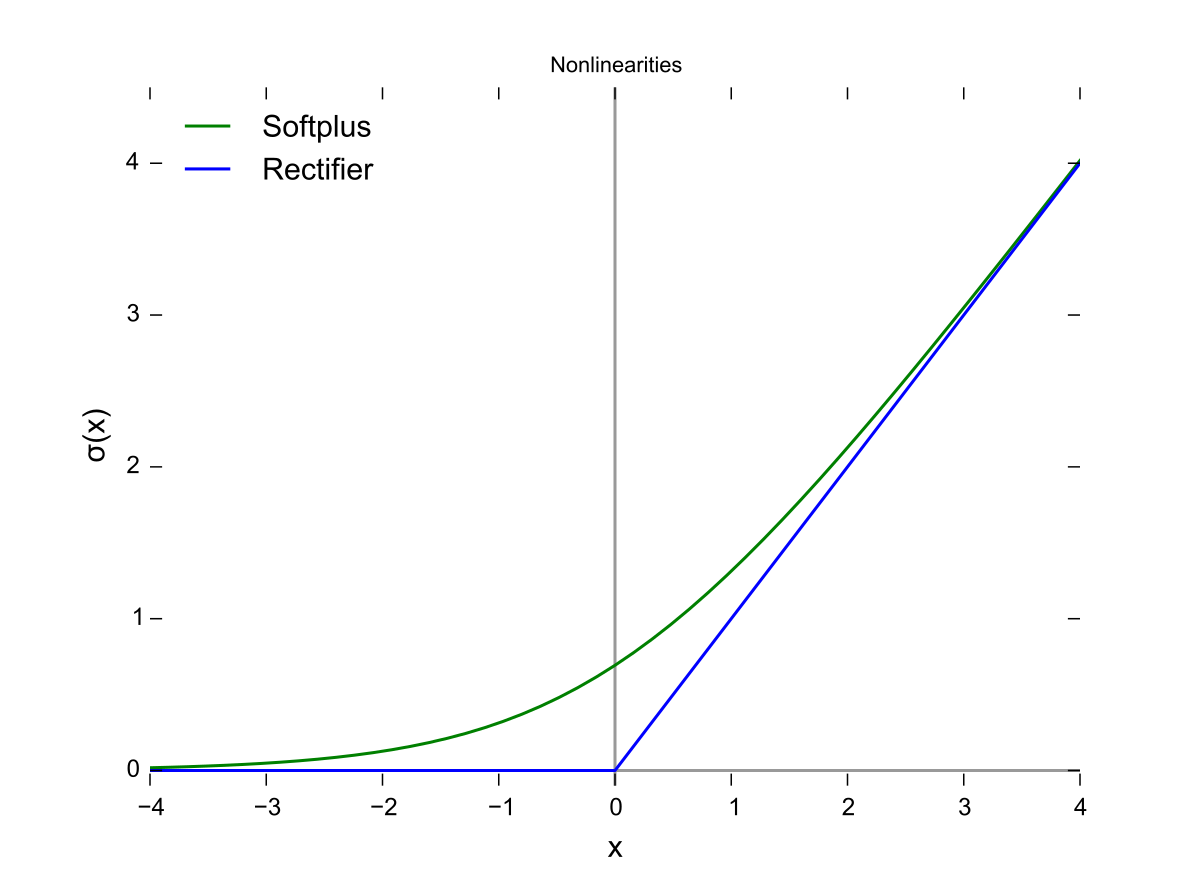
Softmax (for multi-class classification): \(\sigma(\mathbf{x})_i = \frac{e^{x_i}}{\sum_{j} e^{x_j}}\)

If we have two outputs, then the softmax becomes the sigmoid.

Convolutional Neural Networks (CNNs)

The Convolution Operation

The issue with fully connected layers is that they are sensitive to the location of the feature in the data. If our trainig data always shows birds in the sky, then the model will learn to only classify birds in the top half of the image.

This is where convolutional layers come in. Like fully connected layers convolutional layers are a type of layer that is used to extract features from the data. But they are invariant to the location of the feature in the data. They do this by using a filter/kernal which is a small matrix of weights that we slide over the image to get the feature.

\(Y(i, j) = \sum_m \sum_n K(m, n) X(i - m, j - n)\) where:

$X(i,j)$ is the input pixel,
$K(m,n)$ is the filter,
$Y(i,j)$ is the output at position $(i,j)$.

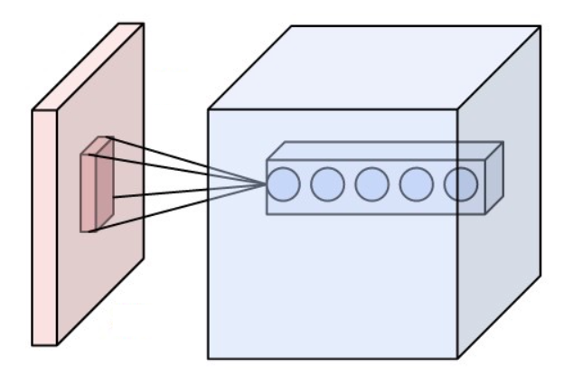
Figure: A visual representation of the convolution operation. The filter (kernel) is applied to the input image, resulting in an output feature map. Image from Wikimedia Commons.

Pooling Layers:
Max Pooling:

ResNet: Deep Residual Networks

One issue that happens when you train a neural network is that the gradient (our signal on how to change the parameters) can become 0, meaning we can’t learn anything. To get around this, ResNet introduced residual connections. These are basically a shortcut from the input to the output. It’s quite amazing about how successful they were, basically every model pre-2022 used some sort of skip connection.

\(\mathbf{y} = F(\mathbf{x}) + \mathbf{x}\) A basic ResNet block is:

i.e. we basically add the input to the output, this allows the gradient to flow directly through the network.

Figure: A ResNet block showing the skip connection (shortcut) that allows gradients to flow directly through the network. The main path consists of convolutional layers with batch normalization and ReLU activation. Image from He et al. 2015

U-Net

The other popular architecture in the field of computer vision is U-Net. It’s a type of convolutional neural network that is used when we want the output to have the same size as the input. It’s a type of encoder-decoder architecture. It basically consists of a contracting path and an expanding path.

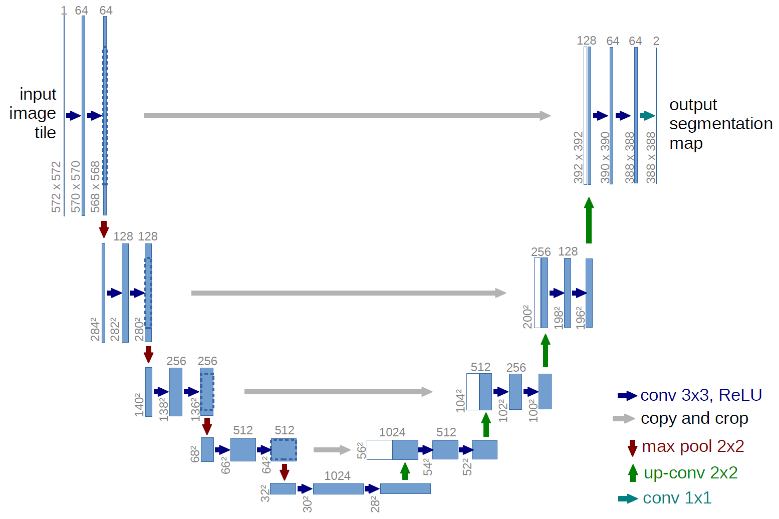
Figure: U-Net architecture showing the contracting path (left) and expansive path (right). Image from Ronneberger et al. 2015

Training a Neural Network

Training a deep neural network involves optimizing (finding the best) parameters to minimize a loss function (how wrong the model is). The most common approach is gradient descent.

Loss Function

A typical loss function for classification tasks is the cross-entropy loss:

\(L = - \sum_{i} y_i \log \hat{y}_i\) where:

$y_i$ is the true label,
$\hat{y}_i$ is the predicted probability.

This loss function will return a single number that tells us how wrong the model is. If it is high then the model is doing poorly, if it is low then the model is doing well. We want to find the parameters that minimize this loss function.

Gradient Descent and Backpropagation

Gradient Descent is a method that finds the minimum of a function. It works by taking the gradient of the loss function and then updating the parameters in the opposite direction of the gradient. This is because the gradient points in the direction of the steepest ascent, so by going in the opposite direction we move towards the minimum. A great analogy is if you are on a hill and you want to find the coordinates of the bottom, you look around and take a step in the direction that is steepest downhill. It’s the same with optimizing a neural network, we want to find the parameters that minimize the loss function, rather than the coordinates of the bottom of the hill.

The weight update rule in gradient descent:

Like walking down the hill, we take several steps in the direction that is steepest downhill.

Algorithm: Gradient Descent

Input: Training data ${\mathbf{X}, \mathbf{y}}$, learning rate $\eta$, max epochs $T$, convergence threshold $\epsilon$

Output: Optimized parameters $\mathbf{w}$

Algorithm:

1. Initialize $\mathbf{w}^{(0)}$ randomly
2. Set $t = 0$
3. While $t < T$:
   1. Forward pass:
      • Compute predictions: $\hat{\mathbf{y}} = f(\mathbf{X}; \mathbf{w}^{(t)})$
      • Compute loss: $L^{(t)} = -\sum_i y_i \log \hat{y}_i$
   2. Backward pass:
      • Compute gradients: $\mathbf{g}^{(t)} = \nabla_{\mathbf{w}} L(\mathbf{w}^{(t)})$
   3. Update parameters:
      • $\mathbf{w}^{(t+1)} = \mathbf{w}^{(t)} - \eta \mathbf{g}^{(t)}$
   4. $t = t + 1$
4. Return $\mathbf{w}^{(t)}$

Note: The convergence check starts after the first iteration ($t > 0$) since $L^{(t-1)}$ doesn’t exist for $t=0$.

Here epochs is the number of times we pass through the data. and $\eta$ is the learning rate that controls how big of a step we take in the direction of the gradient.

Summary

That’s it! You now know the fundamental building blocks of deep learning. In the next blog post we will dig more into the math and details of why this works.

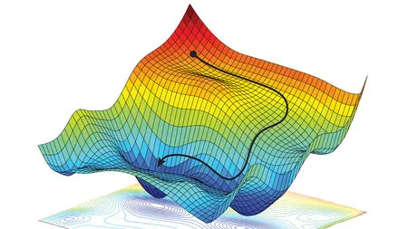
In the last post we spoke about walking down the hill to find the location of the lowest point. This is a great analogy for training a neural network, we want to find the parameters that minimize the loss function. You can think of the loss function as the height of the hill, and the parameters as the coordinates of the hill. This landscape is called the loss landscape, and we talk alot about it in the deep learning community. Specifically in relation to valleys, local minima, saddle points, and flat regions. Whenever you hear these terms, just think about hills and valleys.

Here’s a visualization of a real neural network’s loss landscape:

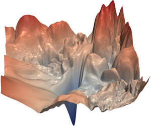
This visualization comes from the paper “Visualizing the Loss Landscape of Neural Nets” (Li et al., 2018). The plot shows the loss surface of a ResNet-56 neural network trained on CIFAR-10. The valleys, peaks, and contours represent different loss values as the network’s parameters change. The relatively smooth areas indicate regions where training can proceed effectively, i.e. you can walk down the hill. But the the sharp peaks and valleys show areas where training might become unstable, i.e. you would fall off a cliff. This kind of visualization has been instrumental in understanding why deep neural networks can be challenging to train and why certain architectures train more successfully than others.

Training Dynamics

When training neural networks, we encounter various phenomena that affect how well and how quickly the network learns. Let’s explore some key concepts in training dynamics:

Local Minima and Global Minima

A local minimum is a point where the loss is lower than all nearby points, but may not be the lowest possible value (global minimum). Early concerns about local minima hampering neural network training have largely been addressed by research showing that in high-dimensional spaces, most local minima are actually quite good solutions. The real challenge often lies elsewhere.

The figure above shows a 2D loss landscape with both local and global minima. The local minimum represents a point where the loss is lower than its immediate surroundings but not the lowest possible value. The global minimum represents the lowest possible loss value in the entire landscape. In practice, neural networks operate in much higher dimensional spaces, but this 2D visualization helps build intuition about these important concepts.

Saddle Points

Saddle points are locations where the gradient is zero, but they’re neither minima nor maxima - imagine a mountain pass between two peaks. These are actually more common than local minima in high-dimensional spaces and can significantly slow down training as optimizers can get “stuck” here temporarily. This is one reason why momentum-based optimizers are helpful - they can help push through these flat regions.

A saddle point in 3D, showing the characteristic “mountain pass” shape. From one direction it looks like a maximum (going up), while from another direction it looks like a minimum (going down). This geometry makes it challenging for optimizers, as the gradient is zero at this point despite it not being a minimum.

Gradient Issues

Several gradient-related challenges can affect training:

1. Vanishing Gradients: When gradients become extremely small, parameters barely update, making learning very slow or impossible. This often happens in deep networks, especially with certain activation functions like sigmoid. Here we can be at a local minimum, but it’s a very bad one. This if often why we use ReLU activation functions.

2. Exploding Gradients: The opposite problem - when gradients become very large, causing unstable training with dramatic parameter updates, like falling off a cliff. This can make the network “bounce” around the loss landscape, never converging to a good solution. This is often why we use gradient clipping, and can be thought of as slowly climbing down the cliff.

Learning Rate Dynamics

The learning rate plays a crucial role in training dynamics:

• Too large: The network might overshoot and lead to a bad outcome, like jumping too far down the hill/cliff
• Too small: Training becomes very slow and might get stuck in poor local optima, we might not be moving fast enough
• Just right: The network converges efficiently to a good solution. Typically we use learning rates that are between 0.001 and 0.00001.

This is why learning rate scheduling (gradually adjusting the learning rate during training) has become a common practice in deep learning.

Jacobian and Hessian in Deep Learning

The Jacobian and Hessian matrices are mathematical tools used to analyze the behavior of the loss landscape. In short they represent the steeness of the loss landscape and how quickly it changes.

Jacobian Matrix

The Jacobian matrix is used to describe the rate of change of the output of a neural network with respect to its inputs, i.e. how steep the loss landscape is at a point. It is particularly useful in understanding how small changes in input can affect the output, which is crucial for tasks like sensitivity analysis and adversarial attacks (more later).

The Jacobian, will give a vector (a direction) of the steepest direction up the loss landscape.

The figure above illustrates the steepness of gradients in a loss landscape. The red regions represent areas with steep gradients where the loss changes rapidly, while the blue regions indicate flatter areas with smaller gradients. Optimizers tend to make larger steps in the steep red regions and smaller steps in the flat blue regions. This visualization helps understand why training can sometimes move quickly through steep areas but slow down significantly in flat regions where the gradients provide less clear directional information. (Image credit: Science Magazine)

Hessian Matrix

The Hessian is a little more confusing, it basically tells you the how quickly the gradient of the loss landscape at a point is changing in any direction. You are right if you’re thinking this sounds a lot like the Jacobian, the Hessian is the Jacobian of the gradient of the loss landscape.

This can be really helpful for analyzing the loss landscape, for example the eigenvalues of the Hessian can indicate the nature of critical points in the loss landscape. Positive eigenvalues suggest a local minimum, negative eigenvalues suggest a local maximum, and mixed signs indicate a saddle point. I.e. it tells you if you are at the bottom of a valley, on top of a peak, or in a flat ridge.

Optimizers

Optimizers are algorithms used to update the parameters of a neural network to minimize the loss function. They play a critical role in the training process. So far we have only used gradient descent, but there are many other optimizers that can be used.

Gradient Descent

The simplest optimizer is gradient descent, which updates parameters in the direction of the negative gradient of the loss function.

Momentum and Adaptive Optimizers

Momentum-based optimizers extend basic gradient descent by incorporating past parameter updates. Think of it like a ball rolling down the hill - it builds up momentum to roll over flat regions and small bumps. The update rule becomes:

Where w are the network parameters, v is the velocity (momentum) term, β controls how much past updates influence the current one, and η is the learning rate.

Adaptive optimizers like Adam go further by maintaining separate learning rates for each parameter. This allows faster progress in directions with consistent gradients while being more cautious in volatile directions. I.e. this is like a ball rolling down the hill, it will pick up speed and be able to roll over small bumps where the landscape is flat, but it will also be able to slow down when it goes down a steep hill.

Adam Optimizer

The Adam optimizer combines momentum with adaptive learning rates. For each parameter w, it tracks:

1. A momentum term $m$ (first moment)
2. A velocity term $v$ (second moment)
3. Bias-corrected versions of both ($\hat{m}$ and $\hat{v}$)

The full update equations are:

Where $\beta_1$ and $\beta_2$ control the decay rates of the momentum and velocity terms respectively, and $\epsilon$ is a small constant for numerical stability. This adaptive approach has made Adam and its variants the go-to optimizers in modern deep learning, thanks to the pioneering work of Diederik Kingma and Jimmy Ba, who in my opinion don’t get enough credit for their work on this.

Summary

Hope this was helpful, I imagine it’s a lot to take in but it’s important to start thinking and understanding what is actually happening when we train a neural network. In the next post we’ll be looking at generative models, early verions of diffusion models for image generation.

The main goal of generative model is the ‘generate’ some new data, unlike in classification where we have a fixed set of classes we want to predict. It’s basically producing rather than predicting. There are four main types of generative models: VAEs, GANs, Normalizing Flows, Invertible Neural Networks and Diffusion Models (for next time), and they all try and learn a model which captures the underlying structure of the data.

Fitting a Normal Distribution to Data

Before diving into fancy generative models, let’s build some intuition by considering a simple example, fitting a normal distribution (bell curve) to some data. Let’s say we have a dataset of heights of people in a population. We can model this as a normal distribution, which is defined by two parameters: the mean $\mu$ and the variance $\sigma^2$, and is given by:

Steps to fit a normal distribution to data:

1. Estimate the mean ($\mu$) and variance ($\sigma^2$): Given a dataset ${x_1, x_2, \ldots, x_n}$, the mean and variance are computed as: \(\mu = \frac{1}{n} \sum_{i=1}^{n} x_i, \quad \sigma^2 = \frac{1}{n} \sum_{i=1}^{n} (x_i - \mu)^2\)

2. Maximum Likelihood Estimation (MLE): Fitting the distribution using MLE ensures that the chosen parameters (\(\mu\) and \(\sigma\)) maximize the likelihood of the observed data, i.e. the model is most likely to generate the data we observed. This simple fitting procedure sets the foundation for understanding more complex generative models. The loss function for fitting the distribution is:

   \[\mathcal{L} = -\sum_{i=1}^{n} \log p(x_i; \mu, \sigma^2)\]

   where $p(x_i; \mu, \sigma^2)$ is the probability of the $i$-th data point under the normal distribution with parameters $\mu$ and $\sigma^2$. This is very similar to the loss function we use in classification, except here we are fitting a distribution rather than a classifier.

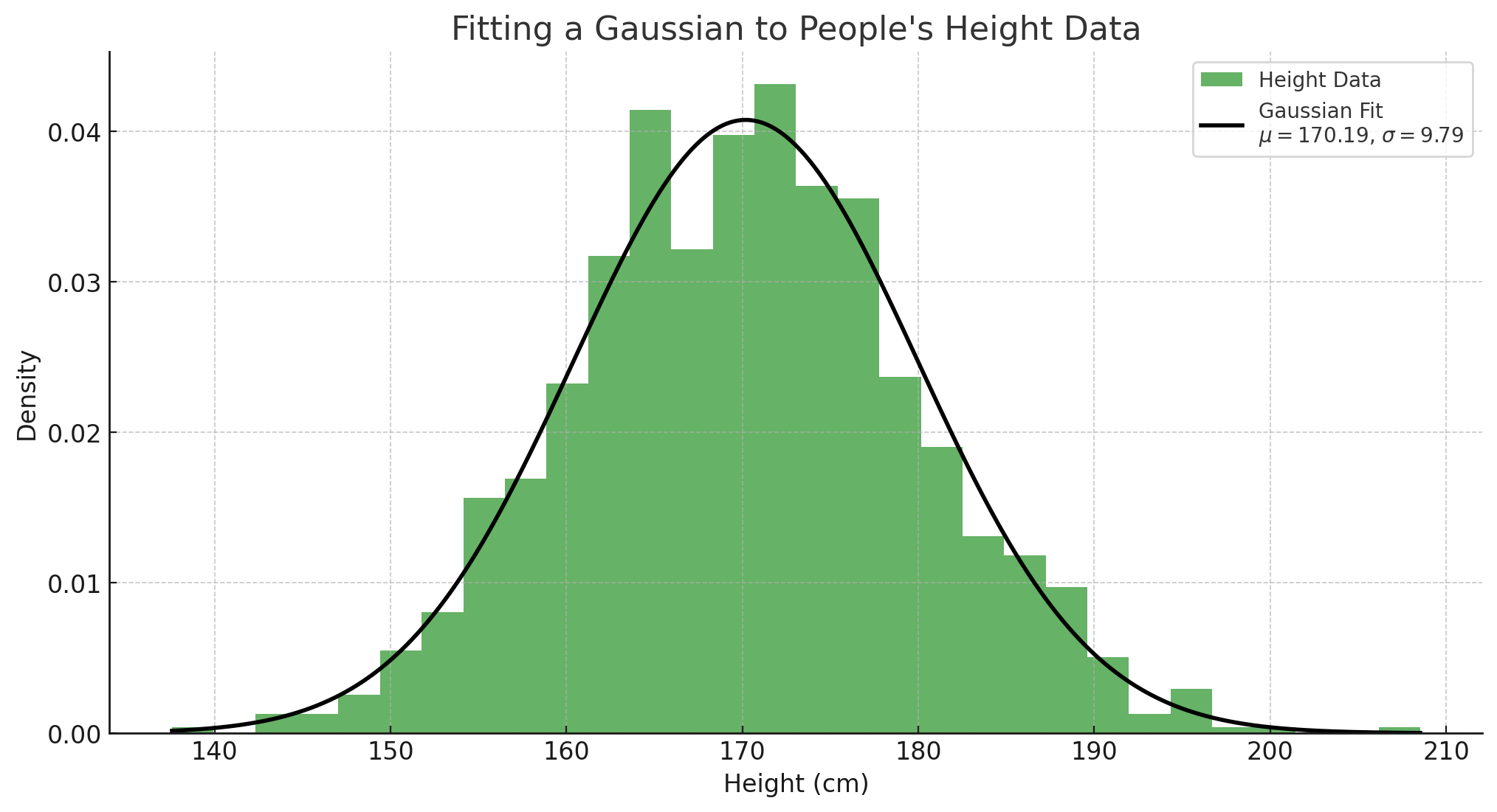
In this section, we visualize the process of fitting a Gaussian distribution to a dataset of heights. The goal is to estimate the mean ($\mu$) and standard deviation ($\sigma$) of the heights in the population.

The mean represents the average height, while the standard deviation indicates how much the heights vary from the mean. By fitting a Gaussian distribution, we can see how well our model captures the underlying data distribution. The curve illustrates the probability density function of the fitted normal distribution, showing the likelihood of different height values occurring in the population. This foundational concept is crucial for understanding more complex generative models that build upon the principles of normal distributions.

The loss landscape here will be a two dimensional one, with the two dimensions being the mean and the variance. We could do gradient descent on this landscape to find the optimal parameters, but we can actually find with a bit of maths that we end up with the closed form solution for the mean and variance. It’s worth trying to do this, hint take the gradient and set it to 0, then solve for \(\mu\) and \(\sigma\).

The Manifold Hypothesis

In high-dimensional spaces (like an image), data rarely lies in a simple Gaussian distribution, instead it’s in a much more complex distribution. The manifold hypothesis is a key idea in generative modeling, suggesting that high-dimensional data (like images or audio) lies on a lower-dimensional manifold (surface) embedded within the high-dimensional space. An intuitive way to think about is this is that there many combinations of pixels that form an image, but only some of those combinations look like images.

For example: A 64x64 image of a face lives in a 4,096-dimensional space, but the set of all possible human faces occupies a much smaller subspace. Generative models aim to learn this underlying manifold and generate new samples that also lie on it. This hypothesis is crucial for models like GANs and VAEs, which seek to capture the data’s latent structure - the underlying characteristics such as shape, colour, etc, and not just the pixel values.

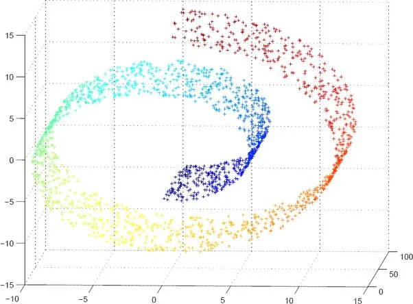
This image illustrates the manifold hypothesis, which shows that high-dimensional data lies on a lower-dimensional manifold within the high-dimensional space. i.e. a 2d plane in a 3d space.

Generative Adversarial Networks (GANs)

GANs, introduced by Goodfellow et al. in 2014, are a class of generative models that learn to generate data by playing a minimax game between two neural networks:

• Generator (G): Generates fake samples from random noise.
• Discriminator (D): Distinguishes between real and fake samples.

Objective Function (Minimax Game): The goal is to learn a generator that fools the discriminator and a discriminator that can tell the difference between a real and fake images, this is basically an arms race. The GAN objective can be expressed as: \(\min_G \max_D \mathbb{E}_{x \sim p_{data}} [\log D(x)] + \mathbb{E}_{z \sim p_z} [\log (1 - D(G(z)))]\)

We basically try and train both the generator and discriminator to get better at their respective tasks. The generator is trying to generate samples that are indistinguishable from the real data, while the discriminator is trying to correctly classify real and fake samples. You might have noticed that the descriminator is using the Binary Cross Entropy loss, while the generator if folliwng the example above.

Lipschitz Continuity and WGANs:

A significant challenge with GANs is training stability. As we spoke about last time, this is caused by loss landscape not being smooth enough, leading to exploding gradients. To get around this, we can enforce the Lipschitz (basically tells you the maximum gradient) constraint on the discriminator. This is done by clipping the weights of the discriminator, or using a gradient penalty.

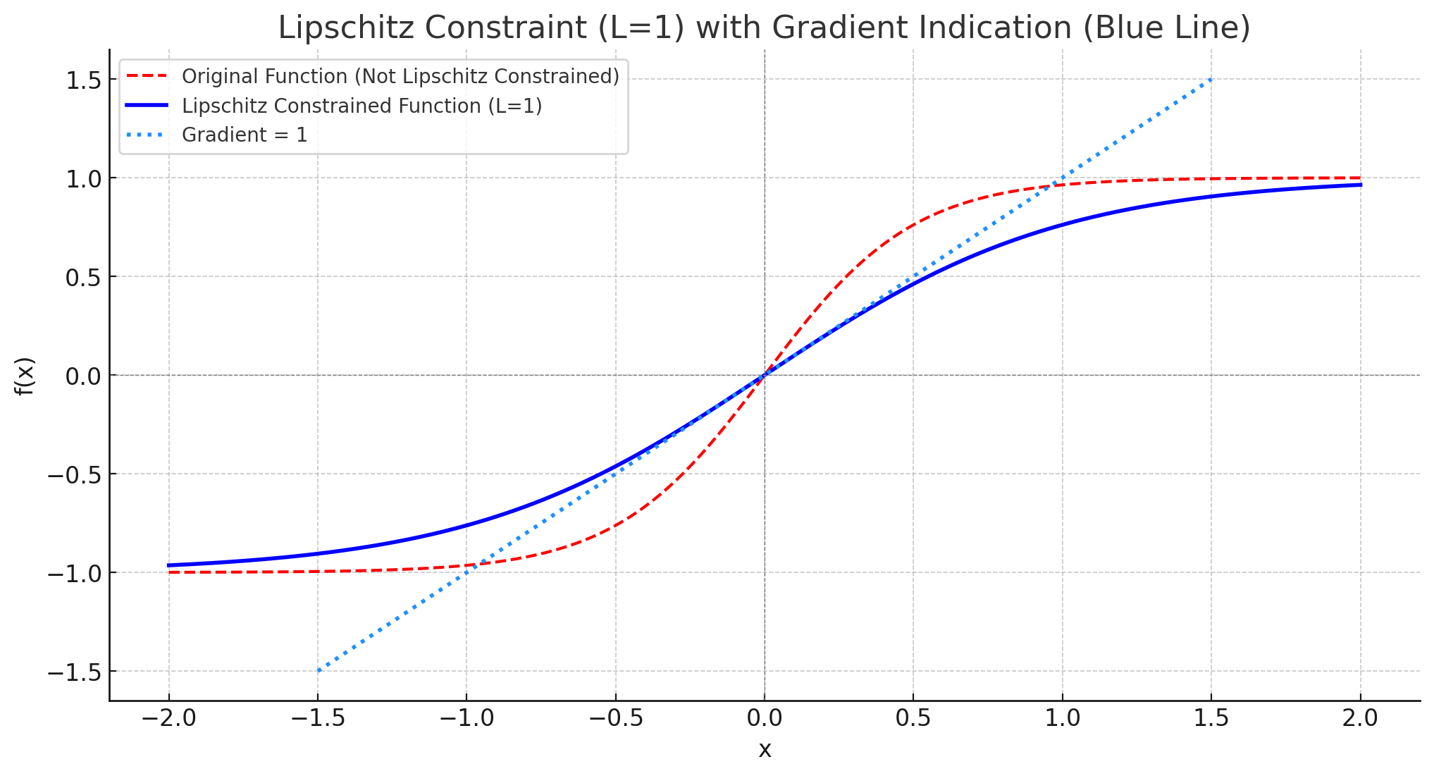
Lipschitz continuit is important as the gradients are bounded, if a function is Lipschitz continuous with a constant ( L ), it means that the absolute value of the gradient is at most ( L ). In our case, if we enforce a Lipschitz constraint of 1, it implies that the gradients of the discriminator in the GAN setup cannot exceed 1. This helps in stabilizing the training process, preventing issues like exploding gradients, and ensures that the updates to the model parameters remain controlled and manageable, i.e we don’t fall of a cliff.

Improved Techniques for GANs:

• WGAN: A method that enforces the Lipschitz constraint by clipping the weights of the discriminator.
• WGAN-GP: A smooth way to enforce the Lipschitz constraint, i.e. we don’t do hard clipping.
• Spectral Normalization: Ensures Lipschitz continuity by normalizing the spectral norm of each layer.
• Orthogonal Weights: Use orthogonal weights, this is isn’t neceesarily related to Lipshitz, but it helps keep the samples diverse by stopiing the representations collapsing to a lower dimensional feature space (i.e. we have many more features to play with).

Variational Autoencoders (VAEs)

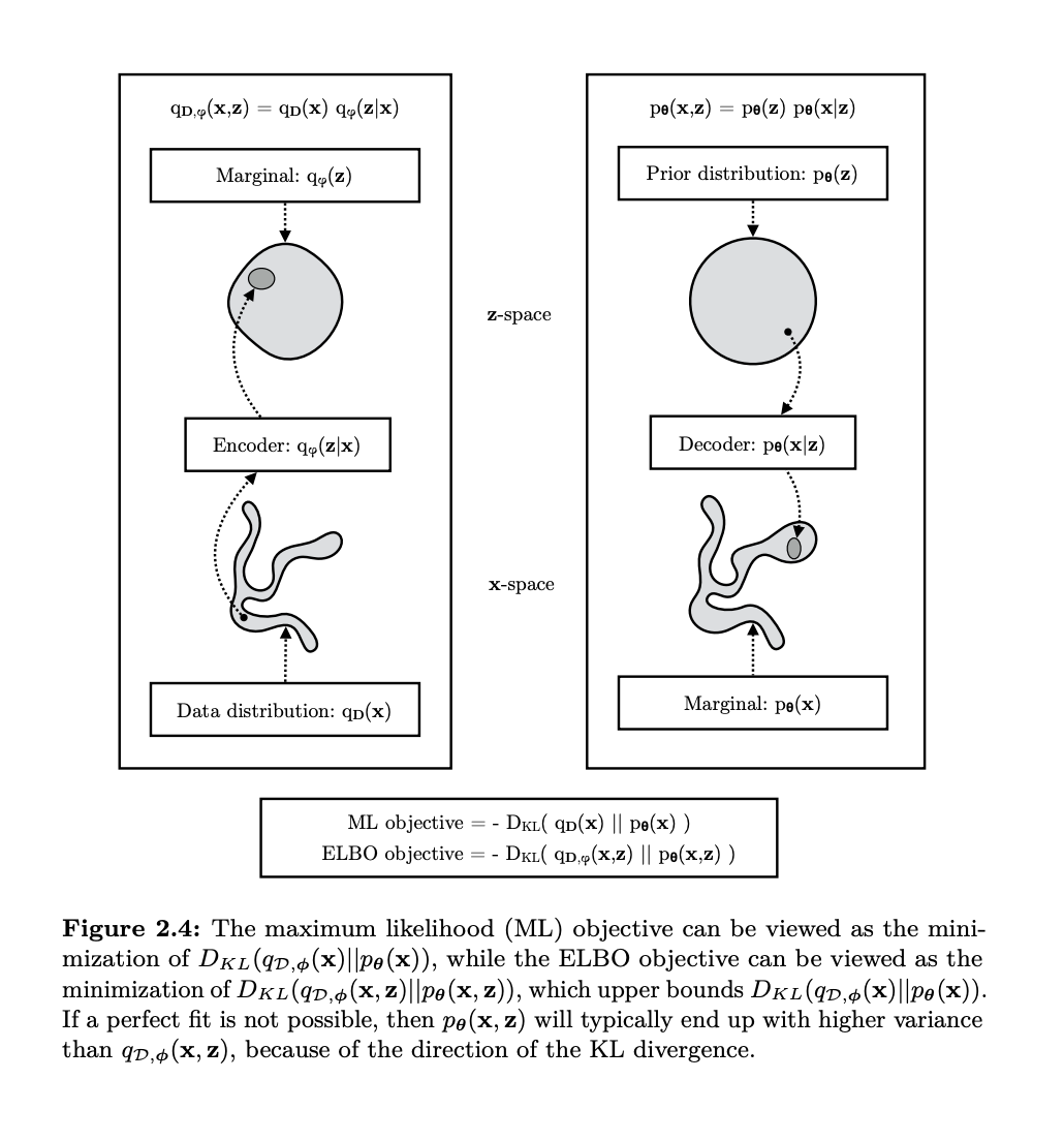
Variational Autoencoders (VAEs) are another type of generative models that combine probabilistic modeling with neural networks. Unlike GANs, which generate data adversarially, VAEs take a probabilistic approach to model the latent space, i.e. they try and fit a distribution to the data, but also try and learn the latent factors. The core idea is to encode input data into a probabilistic distribution over a latent space and then decode it back to generate samples. This is a great example of how we want to map from the simple distribution containing the latent factors to the complex distribution containing the data.

Key Concepts in VAEs

The Evidence Lower Bound (ELBO)

The VAE maximizes a lower bound on the data likelihood known as the Evidence Lower Bound (ELBO). We can derive the ELBO like so:

1. Start with the definition of the marginal likelihood, i.e. margincalize out \(z\): \(p(x) = \int p(x|z) p(z) dz\)

2. Introduce an approximate posterior \(q(z \mid x)\): \(p(x) = \int q(z|x) \frac{p(x|z) p(z)}{q(z|x)} dz\)

3. Apply Jensen’s inequality (this is where the lower bound comes in): \(\log p(x) \geq \mathbb{E}_{q(z|x)}\left[\log \frac{p(x|z) p(z)}{q(z|x)}\right]\)

4. This can be rewritten as: \(\log p(x) \geq \mathbb{E}_{q(z|x)}[\log p(x|z)] - D_{KL}(q(z|x) || p(z))\)

5. Thus, we arrive at the final form of the ELBO: \(\log p(x) \geq \mathbb{E}_{q(z|x)}[\log p(x|z)] - D_{KL}(q(z|x) || p(z))\)

Here, \(q(z\mid x)\) is the approximate posterior, and \(D_{KL}\) is the Kullback-Leibler divergence, which penalizes deviations of \(q(z\mid x)\) from the prior \(p(z)\). The reconstruction term encourages accurate reconstructions of the input, while the KL divergence term ensures a structured latent space. Mechanistically, we first encode \(\x\) through \(q(z\mid x)\), which is a neural network that predicts a meand and variance, we sample from this Gaussian distribution and then reconstruct the sample. We then take the mean squared error between the input \(x\) and the the output form the decoder, which is just summing up the difference between the pixels, taking the square and then dividing by the number of pixels.

Variance of the Estimators and Gradient Stability

In the context of VAEs, high variance in the gradient estimate to the encoder arise when sampling from the approximate posterior \(q(z|x)\), as it’s a stochastic process (think about randomly changing your directioin while walking down the hill). Since backpropagation cannot flow through random sampling, techniques like REINFORCE or the reparameterization trick are necessary to ensure stable training.

REINFORCE and Variance in Gradient Estimators

REINFORCE is a fundamental algorithm in reinforcement learning (Williams, 1992) but is also applicable in probabilistic models like VAEs. It provides an unbiased gradient estimator for expectations over stochastic processes, but this estimator often suffers from high variance, making training challenging and unstable.

For a probability distribution parameterized by \(\theta\), the goal is to compute the gradient of an expectation:

(For a VAE we’re trying to compute the gradient of the ELBO, so we’re trying to compute the gradient of the expectation of the log likelihood of the data under the model. Using the log-derivative trick, REINFORCE estimates the gradient as:

This is an unbiased estimator (i.e. on average it gets to the true value), but the variance of the estimator can still be very high.

The Reparameterization Trick

This is the most common solution to high variance in VAEs, transforming the stochastic sampling process into a deterministic one by introducing auxiliary noise:

By reparameterizing, gradients can propagate through \(\mu(x)\) and \(\sigma(x)\) directly, i.e. we take the gradient of the mean and variance directly and not the same, this reduces the variance and allows us to train the model.

Variance Reduction with Control Variates

Borrowing from reinforcement learning, control variates can further reduce variance. A baseline function can be subtracted from the reward signal without introducing bias, stabilizing training. For example, a learned value function \(b(x)\) can serve as a baseline:

KL Annealing

Gradually increasing the weight of the KL divergence term (annealing) during early training prevents the model from collapsing the latent space too soon (posterior collapse), leading to more stable and meaningful representations.

Intepretability of VAEs

One of the main reason people like VAEs is that we can use the latent space to interpret features of the data. For example, if we have a VAE that models human faces, we can use the latent space to understand how different features of the face are related to each other. We can also change the latent factors and directly cause certain features to change in the image. This can be seen in the image below:

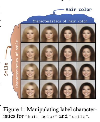
This is really useful when compared to GANs, as we can now theoretically control conceptual factors of the image by altering certain parts of the latent space.

Invertible Neural Networks (INNs)

Invertible Neural Networks (INNs) focus on learning bijective (one to one) transformations between the data space and the latent space. Unlike VAEs and GANs, INNs ensure exact likelihoods. They are similar to the VAE in that they map compelx data to a latent space, but they are different in that they are invertible, i.e. there is not fixed decoder/encoder, it is just one network that maps forwards and backwards. They start by modelling a change of variables:

which when taking the log for high dimensional data, we get:

where $z$ is the latent space and $x$ is the data space, and the final term is the log determinant of the Jacobian matrix of the transformation.

• Rank and Lipschitz Constraints: As we are dealing with Jacobians (gradient of all outputs wrt to all inputs), we need to ensure that the transformation is bijective, i.e. one-to-one and invertible. Controlling the Lipschitz constant helps maintain stability and ensures smooth transformations. A great way to do this is through the use of ResNets, which due to their skip connections are always full rank and invertible. Check out the paper Invertible Residual Networks for more details.

Summary

Each of these generative models—GANs, VAEs, and INNs—offers unique advantages and challenges. The choice of model depends on the task at hand:

• GANs are best for generating high quality images (pre diffusion models).
• VAEs are best for finding the latent features.
• INNs offer exact computation of the likelihood.

Most of these methods are now obsolete, and have been replaced by more powerful methods such as diffusion models, which we will cover next time.