| CARVIEW |
We recall that a periodic point of period 


Theorem 1. (Sharkovsky’s “little” theorem) Let 


Note that no hypothesis is made on 
Our proof of Sharkovsky’s “little” theorem follows the one given in (Sternberg, 2010), and could even be given in a Calculus 1 course: the most advanced result will be the intermediate value theorem.
Lemma 1. Let ![I=[a,b]](https://s0.wp.com/latex.php?latex=I%3D%5Ba%2Cb%5D&bg=ffffff&fg=333333&s=0&c=20201002)


Proof. Let 


Lemma 2. In the hypotheses of Lemma 1, let 


Proof. Let ![K=[c,d]](https://s0.wp.com/latex.php?latex=K%3D%5Bc%2Cd%5D&bg=ffffff&fg=333333&s=0&c=20201002)


- There exists
such that
. Let
, and let
. Then surely
, but if for some
we had either
or
, then by the intermediate value theorem, for some
we would also have either
or
, against our choice of
for every
be the largest
such that
. Then
Proof of Sharkovsky’s “little” theorem. Let 


Let ![L=[a,b]](https://s0.wp.com/latex.php?latex=L%3D%5Ba%2Cb%5D&bg=ffffff&fg=333333&s=0&c=20201002)
![R=[b,c]](https://s0.wp.com/latex.php?latex=R%3D%5Bb%2Cc%5D&bg=ffffff&fg=333333&s=0&c=20201002)
![[a,c]](https://s0.wp.com/latex.php?latex=%5Ba%2Cc%5D&bg=ffffff&fg=333333&s=0&c=20201002)


By Lemma 2, there exists a closed and bounded subinterval 


We stop at 


Can the least period of 


![i\in[2:n]](https://s0.wp.com/latex.php?latex=i%5Cin%5B2%3An%5D&bg=ffffff&fg=333333&s=0&c=20201002)


Theorem 1 is a special case of a much more general, and complex, result also due to Sharkovsky. Before stating it, we need to define a special ordering on positive integers.
Definition. The Sharkovsky ordering 
- Identify the number
, with
.
- Sort the pairs with
in lexicographic order.
That is: first, list all the odd numbers, in increasing order; then, all the doubles of the odd numbers, in increasing order; then, all the quadruples of the odd numbers, in increasing order; and so on.
For example,and
- Set
for every
.
That is: the powers of 2 follow, in the Sharkovskii ordering, any number which has an odd factor.
For example,.
- Sort the pairs of the form
—i.e., the powers of 2—in reverse order.

The set of positive integer with the Sharkowsky ordering has then the form:

Note that
Theorem 2. (Sharkovsky’s “great” theorem) Let 
- If
, then
- For every
integer it is possible to choose
. In particular, there are functions whose only periodic points are fixed.
Bibliography:
- Keith Burns and Boris Hasselblatt. The Sharkovsky theorem: A natural direct proof. The American Mathematical Monthly 118(3) (2011), 229–244. doi:10.4169/amer.math.monthly.118.03.229
- Robert L. Devaney, An Introduction to Chaotic Dynamical Systems, Second Edition, Westview Press 2003.
- Shlomo Sternberg, Dynamical Systems, Dover 2010.
Find the talk on my personal blog HERE
]]>Let’s start from the beginning:
Definition 1. Let 


If 


Usually, we will have 


Examples of subadditive functions are:
- The Heaviside function
defined by
if
and
if
. This function is subadditive, because if
are both negative, then the left-hand side of (1) is 0, and if one of them is nonnegative, then the right-hand side is either 1 or 2.
- Let
and let
if
and
if
. Then
and
this shows that a subadditive function can be discontinuous at every point.
- Let
be a finite nonempty set and let
be the free monoid on
as the identity element. The length of a word is a subadditive (actually, additive) function on
If 


Fekete’s lemma. Let
- If
or
, then
.
- Dually, if
or
, then
.
- Finally, if
, then
, and both are finite.
Note that 


Proof of point 1 with 


But by construction, 


This holds for every positive integer

A key ingredient of the proof is that 

An immediate consequence of Fekete’s lemma is that, as it was intuitively true from the definition, a subadditive function defined on 
Lemma 1. Let 

Proof: If 


Hence, if 


To see an application of Fekete’s lemma in the context of the theory of dynamical system, we introduce the notions of subshift and of cellular automaton. We will first do so in dimension 1, then expand to arbitrary dimension in later talks.
Definition 2. Let 


Examples of subshifts are:
- The full shift
. In this case,
.
- The golden mean shift on the binary alphabet, where
.
Let 

is a subadditive function of the positive integer variable
exists. The quantity (2) is called the entropy of the subshift
(As a funny note, the use of the uncapitalized letter 


Definition 3. A one-dimensional cellular automaton is a triple 


A cellular automaton 
If 

In the upcoming talk (or talks) we will examine the case of several variables, and correspondingly, subshifts and cellular automata in higher dimension. In particular, we will discuss a generalization of Fekete’s lemma to arbitrarily many positive integer variables.
Bibliography:
- Silvio Capobianco. Multidimensional cellular automata and generalization of Fekete’s lemma. Discrete Mathematics and Theoretical Computer Science 10 (2008), 95–104.
- Einar Hille. Functional Analysis and Semigroups. American Mathematical Society, 1948.
- Douglas Lind and Brian Marcus. An Introduction to Symbolic Dynamics and Coding. Cambridge University Press 1995.
- Tommaso Toffoli, Silvio Capobianco, and Patrizia Mentrasti. When—and how—can a cellular automaton be rewritten as a lattice gas? Theoretical Computer Science 403 (2008), 71–88.
First of all, let us recall what the Church-Turing thesis is, and what it is not. Its statement, as reported by the Stanford Encyclopedia of Philosophy, goes as follows:
A function of positive integers is effectively calculable only if recursive.
Here, for a calculation procedure to be “effective” means the following:
- it has a finite description;
- it always returns the correct output, given any valid input;
- it can be “carried on by pencil and paper” by a human being; and
- it requires no insight or ingenuity on the human’s behalf.
One model of effective procedures is given by the recursive functions; another one, by the functions computable by Turing machines; a third one, by the functions which are representable in Church’s
The class of Turing machines has the advantage of containing a universal element: a special Turing machine and an encoding from the set of Turing machines to the set of natural numbers exists such that, when the special Turing machine is provided the encoding of an arbitrary Turing machine and a valid input for the latter, it will return the value of the encoded Turing machine on the provided input.
Now that we have written down what the Church-Turing thesis is, we can examine Akl’s theorem.
In his 2005 paper, Akl defines a universal computer as a system 
- It has means of communicating with the outside world, so to receive input, and where to send its output.
- It can perform every elementary arithmetic and logic operations.
- It can be programmed, according to the two previous rules.
- It has unlimited memory to use for input, output, and temporary values.
- It can only execute finitely many operations (evaluating input, producing output, performing an elementary operation, etc.) at each time step.
- It can simulate any computation performed by any other model of computation.
The statement of the theorem, which does not appear explicitly in the original paper but is written down in the one from 2015 which clarifies the idea and addresses criticism, is hereby reported verbatim:
Nonuniversality in Computation Theorem (NCT): No computer is universal if it is capable of exactly 

The main argument is that no such computer can perform a computation which requires more than 
Such requirement, however, does not appear in the notion of universality at the base of the original, and actual, Church-Turing thesis. There, to “simulate” a machine or algorithm means to be able of always reproducing the same output of the algorithm, given any valid input for it, up to an encoding of the input and the output. But no hypothesis on how the output is achieved from the input is made: a simulation in linear time, such that each step of the simulated algorithm is reproduced by exactly 
Among the (counter)examples provided by Akl are:
- Computations with time-varying variables.
- Computations with time-varying computational complexity.
- Computations whose complexity depends on their placement on a schedule.
- Computations with interacting variables, e.g., states of entangled electrons.
- Computations with uncertain time constraints.
None of these, however, respect the definition of computation from the model of recursive functions: where the values of the variables are given once and for all, and can possibly change for recursive calls, but not for the original call. They can be seen as instances of unconventional models of computation: but by doing this, one changes the very notion of computation, which ceases to be the one at the basis of the Church-Turing thesis.
So my guess is that Akl’s statement about the falsity of the Church-Turing thesis actually falls in the following category, as reported in the humorous list by Dana Angluin:
Proof by semantic shift: Some standard but inconvenient definitions are changed for the statement of the result.
Actually, if we go back to Akl’s definition of a universal computer, it appears to be fine until the very last: the first two points agree with the definition of effective computation at the basis of the actual Church-Turing thesis, the next three are features of any universal Turing machine. The problem comes from the last point, which has at least two weak spots: the first one being that it does not define precisely what a model of computation is, which can be accepted as Akl is talking of unconventional computation, and it is wiser to be open to other possibilities. But there is a more serious one, in that it is not clear
what does the expression “to simulate” mean.
Note that the Stanford Encyclopedia of Philosophy reports the following variant of the Church-Turing thesis, attributed to David Deutsch:
Every finitely realizable physical system can be perfectly simulated by a universal model computing machine operating by finite means.
Deutsch’s thesis, however, does not coincide with the Church-Turing thesis! (This, notwithstanding Deutsch’s statement that “[t]his formulation is both better defined and more physical than Turing’s own way of expressing it”.) Plus, there is another serious ambiguity, which is of the same kind as the one in Akl’s definition:
what is “perfectly simulated” supposed to mean?
Does it mean that every single step performed by the system can be reproduced in real time? In this case, Akl is perfectly right in disproving it under the constraint of boundedly many operations at each time unit. Or does it mean that the simulation of each elementary step of the process (e.g., one performed in a quantum of time) ends with the correct result if the correct initial conditions are given? In this case, the requirement to reproduce exactly what happens between the reading of the input and the writing of the output is null and void.
Worse still, there is a vulgarized form of the Church-Turing thesis, which is reported by Akl himself on page 172 of his 2005 paper!, and goes as follows:
Any computable function can be computed on a Turing machine.
If one calls that “the Church-Turing thesis”, then Akl’s NCT is absolutely correct in disproving it. But that is not the actual Church-Turing thesis! It is actually a rewording of what in the Stanford Encyclopedia of Philosophy is called “Thesis M”, and explicitly stated not to be equivalent to the original Church-Turing thesis—and also false. Again, the careful reader will have noticed that, in the statement above, being “computable by a Turing machine” is a well defined property, but “computable” tout court definitely not so.
At the end of this discussion, my thesis is that Akl’s proof is correct, but NCT’s consequences and interpretation might not be what Akl means, or (inclusive disjunction) what his critics understand. As for my personal interpretation of NCT, here it goes:
No computer which is able to perform a predefinite, finite number of operations at each finite time step, is universal across all the different models of computation, where the word “computation” may be taken in a different meaning than that of the Church-Turing thesis.
Is mine an interpretation by semantic shift? Discussion is welcome.
References:
- Selim G. Akl. The Myth of Universal Computation. Parallel Numerics ’05, 167–192.
- Selim G. Akl. Nonuniversality explained. International Journal of Parallel, Emergent and Distributed Systems 31:3, 201–219. doi:10.1080/17445760.2015.1079321
- The Church-Turing Thesis. Stanford Encyclopedia of Philosophy. First published January 8, 1997; substantive revision August 19, 2002. https://plato.stanford.edu/entries/church-turing/
- Dana Angluin’s List of Proof Techniques. https://www.cs.northwestern.edu/~riesbeck/proofs.html
We consider languages made of symbols that represents either objects, or functions, or relations: in particular, unary relations, or equivalently, sets. A sentence on such a language is a finite sequence of symbols from the language and from the standard logical connectives and quantifiers (


For example, the set 


Of course, second-order logic is much more expressive than first order logic. The natural question is: how much?
The answer is: possibly, too much more than we would like.
To discuss how it is so, we recall the notion of model. Informally, a model of a set of sentences is a “world” where all the sentences in the set are true. For instance, the set 
For sets of first-order sentences, the following four results are standard:
Compactness theorem. (Tarski and Mal’tsev) Given a set 
Upwards Löwenheim-Skolem theorem. If a set of first-order sentences has a model of infinite cardinality 

Downwards Löwenheim-Skolem theorem. If a set of first-order sentences on a finite or countable language has a model, then it also has a finite or countable model.
Completeness theorem. (Gödel) Given a set
All of these facts fail for second-order theories. Let us see how:
We start by considering the following second-order sentence:

Lemma 1. The sentence 

The informal reason is that
the universe is a monoid on a single generator
Let us now consider the following second-order sentence:

Lemma 2. The sentence 
The informal reason is that
the universe contains a copy of the natural numbers
Theorem 1. Both Löwenheim-Skolem theorems fail for sets of second-order sentences.
Proof. 

Let us now consider the set 

Clearly, 
Lemma 3. Every model of
The informal reason is that 

Theorem 2. The compactness theorem fails for sets of second-order sentences.
Proof. Let 


We can now prove
Theorem 3. The completeness theorem does not hold for second-order sentences.
In other words, second-order logic is semantically inadequate: it is not true anymore that all “inequivocably true” sentences are theorems. The proof will be based on the following two facts:
Fact 1. (Gödel) The set of the first-order formulas which are true in every model of
Fact 2. (Tarski) The set of first-order formulas which are true in
Fact 1 is actually a consequence of the completeness theorem: the set of first-order formulas which are true in every model of
Proof of Theorem 3. We identify
Let 
Fix a Gödel numbering for sentences. There exists a recursive function that, for every sentence
Suppose now, for the sake of contradiction, that the set of second-order sentences that are true in every model of
Bibliography:
- George S. Boolos et al. Computability and Logic. Fifth Edition. Cambridge University Press, 2007
Given a base 


where each 


and also

Given a nonnegative integer 


- Take the Cantor base-
- Convert each
, getting a new number.
- If the value obtained at the previous point is positive, then subtract
from it.
(This is called the woodworm’s trick.)
Goodstein’s theorem. Whatever the initial value 
Goodstein’s proof relies on the use of ordinal arithmetic. Recall the definition: an ordinal number is an equivalence class of well-ordered sets modulo order isomorphisms, i.e., order-preserving bijections.Observe that such order isomorphism between well-ordered sets, if it exists, is unique: if 


An interval in a well-ordered set 

Fact 1. Given any two well-ordered sets, either they are order-isomorphic, or one of them is order-isomorphic to an initial interval of the other.
In particular, every ordinal 
All ordinal numbers can be obtained via von Neumann’s classification:
- The zero ordinal is
, which is trivially well-ordered as it has no nonempty subsets.
- A successor ordinal is an ordinal of the form
, with every object in
in
.
For instance,can be seen as
.
- A limit ordinal is a nonzero ordinal which is not a successor. Such ordinal must be the least upper bound of the collection of all the ordinals below it.
For instance, the smallest transfinite ordinalis the limit of the collection of the finite ordinals.
Observe that, with this convention, each ordinal is an element of every ordinal strictly greater than itself.
Fact 2. Every set of ordinal numbers is well-ordered with respect to the relation: 

Operations between ordinal numbers are defined as follows: (up to order isomorphisms)
is a copy of
, with every object in
Ifare finite ordinals, then
has the intuitive meaning. On the other hand,
, as a copy of
is strictly larger than
is a stack of
Ifhas the intuitive meaning. On the other hand,
is a stack of
, which is order-isomorphic to
is a stack of
.
is
,
if
, and the least upper bound of the ordinals of the form
with
if
Ifhas the intuitive meaning. On the other hand,
is the least upper bound of all the ordinals of the form
where
.
Proof of Goodstein’s theorem: To each integer value 


and 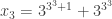


We notice that, in our example, 

At each step 

.
Then,
as
, and
.
and
.
Thenfor a transfinite ordinal
.
.
Thenfor some
, and
is a number whose
th digit in base
.
It is then clear that the sequence 


So why is it that Goodstein’s theorem is not provable in the first order Peano arithmetics? The intuitive reason, is that the exponentiations can be arbitrarily many, which requires having available all the ordinals up to

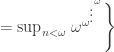
this, however, is impossible if induction only allows finitely many steps, as it is the case for first-order Peano arithmetics. A full discussion of a counterexample, however, would greatly exceed the scope of this post.
]]>Let us recall the basic notions. In a game in normal form we have:
- A set
- A set
of strategies for each player.
- A collection of utility functions
which associate to each strategic profile
a real number, such that
is the utility player
.
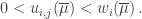
A Nash equilibrium for a game in normal form is a strategic profile 
A mixed strategy for player ![\mu_i : \mathcal{P}(S_i) \to [0,1]](https://s0.wp.com/latex.php?latex=%5Cmu_i+%3A+%5Cmathcal%7BP%7D%28S_i%29+%5Cto+%5B0%2C1%5D&bg=ffffff&fg=333333&s=0&c=20201002)


The idea behind Nash’s proof goes as follows. If the game is finite, then a mixed strategy for player

therefore, mixed strategy profiles can be identified with points of

which is compact and convex as all of its components are. Mixed strategy Nash equilibria are those points of 


Suppose player 

.
.
.
.
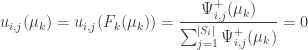
Given 


are continuous and nonnegative and satisfy 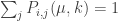

that is,

are continuous transformations of 


Suppose, for the sake of contradiction, that 

Choose 
.
.
.
Points 2 and 3 tells us that 


and as 

To introduce this idea, together with other basic game-theoretic notions, we resort to some examples. Here goes the first one:
Alice and Bob are planning an evening at the cinema. Alice would like to watch the romantic movie, while Bob would like to watch the action movie. Neither of them likes much the other’s favored movie: however, should they split, the sadness for being alone would be so big, that neither of them would enjoy his or her movie!
This is the kind of situation modeled by a game in normal form, where we have:
- A set
- A set
- A collection of utility functions
In the case of Alice and Bob, this may be summarized with a table such as the following:
| Romantic | Action | |
| Romantic |  |
 |
| Action | |
 |
Such tables represent games in normal form between two players, where the rows of the table are labeled with the strategies suitable for the first player, and the columns of the table are labeled with the strategies suitable for the second player: the entries of the table indicate the values of the utility functions when the first player plays the corresponding row and the second player plays the corresponding column. When we want to emphasize the role of player 


Suppose that Alice is the first player, and Bob is the second player: then the table tells us that, if they both choose the romantic movie, Alice will enjoy it a lot (utility value 

Let us consider another game (a rather serious one indeed) where the players are a lion and a gazelle. The lion wants to catch the gazelle; the gazelle wants to avoid being caught by the lion. To do this, they may choose between being on the move, or staying more or less in the same place. It turns out, from observation in the field, that the table for the lion-and-gazelle situation is similar to the one below:
| Move | Stay | |
| Move |  |
 |
| Stay |  |
|
We observe that, for the lion, the most profitable strategy is to move. Indeed, if the gazelle moves, then the utility for the lion is 


So, what if we relax the requirement, and just demand that every player chooses the most favorable strategy, given the strategies of the other players? This is the basic intuition under the concept of Nash equilibrium, formalized and studied by John Nash in his 1950 doctoral thesis.
Definition 1. A Nash equilibrium for a game in normal form is a strategic profile
The situation when both the lion and the gazelle are on the move, is a Nash equilibrium: and is the only Nash equilibrium in the corresponding game. (By definition, every dominant strategy enters every Nash equilibrium.) The situation when both Alice and Bob go watch the romantic movie, is a Nash equilibrium: and so is the one when they go watch the action movie.
So, does every game have a Nash equilibrium?
Actually, no.
Indeed, suppose that the predator and the prey, instead of being large mammals such as the lion and the gazelle, are small insects such as a dragonfly and a mosquito. It then turns out, after careful observation, that the table for the predator-prey game gets more similar to the following:
| Move | Stay | |
| Move |  |
 |
| Stay |  |
 |
In this situation, the dragonfly maximizes its utility if it does the same as the mosquito. In turn, however, the mosquito maximizes its own utility if it does the opposite than the dragonfly! In such a situation there can be no such thing as a Nash equilibrium as defined above.
Where determinism fails, however, randomization may help.
Definition 2. A mixed strategy for the player
For example, the dragonfly might decide to move with probability 

With mixed strategies, the important value for player

which we may write 
Now, suppose that the dragonfly decides to set its own paramenter

which has solution 

which has solution 
Definition 3. A mixed strategy Nash equilibrium for a game in normal form is a mixed strategy profile
And here comes Nash’s great result:
Nash’s theorem. Every game in normal form that allows at most finitely many pure strategic profiles admits at least one, possibly mixed strategy, Nash equilibrium.
It is actually sufficient to prove Nash’s theorem (as he did in his doctoral thesis) when there are only many players, and each of them only has finitely many pure strategies: such limitation is only apparent, because the condition that pure strategy profiles are finitely many means that all players have finitely many pure strategies, and at most finitely many of them have more than one.
The idea of the proof, which we might go through in a future Theory Lunch talk, goes as follows:
- Identify the space of mixed strategic profiles with a compact and convex set
for suitable
- For
.
- By the Brouwer fixed-point theorem, for every
.
- As
- By supposing that
We remark that Nash equilibria are not optimal solutions: they are, at most, lesser evils for everyone given the circumstances. To better explain this we illustrate a classic problem in decision theory, called the prisoner’s dilemma. The police has arrested two people, who are suspects in a bank robbery: however, the only evidence is about carrying firearms without license, which is a minor crime leading to a sentence of one year, compared to the ten years for bank robbery. So, while interrogating each suspect, they propose a bargain: if the person will testify against the other person for bank robbery, the police will drop the charges for carrying firearms without license. The table for the prisoner’s dilemma thus has the following form:
| Quiet | Speak | |
| Quiet |  |
 |
| Speak |  |
 |
Then the situation where both suspects testify against each other is the only pure strategy Nash equilibrium: however, it is very far from being optimal…
]]>I wrote a post on this on my blog on cellular automata.
Link: https://anotherblogonca.wordpress.com/2014/05/15/random-settings-in-cellular-automata-machines/
]]>