A note on the correct definition of a proportion space

Recently I’ve been learning about torsors. A torsor is, in informal terms, an algebraic structure that’s like a group with the identity element “forgotten”. The precise definition (whose connection to the informal notion is not meant to be obvious!) is: a torsor is a set {X} equipped with a group {G} acting on {X} such that for any two elements {a} and {b} of {X}, there is a unique {g \in G} with {ga = b}.

My interest in torsors comes from the idea that the set of all possible values of a dimensional physical quantity, such as mass, is intrinsically a torsor, because the choice of the unit of measurement is arbitrary. Therefore it might make sense to formalize dimensional analysis using the notion of a torsor.

I might have more to say about torsors themselves, and the connection to dimensional analysis, in a future post. But for now, I just want to write about one alternative way of capturing the idea of a “group with the identity element forgotten”, which was described in a blog post by Matt Baker.

Baker introduces the notion of a proportion space, which is a non-empty set {X} equipped with an equivalence relation {(::)} on {X^2} such that:

  1. (PS1) For any two elements {a}, {b} of {X}, we have {(a, a) :: (b,b)}.
  2. (PS2) For any three elements {a}, {b}, {d} of {X}, there is a unique {c \in X} such that {(a, b) :: (c, d)}.

The idea here is that {::} represents a proportion statement, or four-part analogy: for any four elements {a}, {b}, {c}, {d} of {X}, the relation {(a, b) :: (c, d)} is thought of as having the meaning “{a} is to {b} as {c} is to {d}”. Another notation for this meaning which is sometimes seen is

\displaystyle  a : b :: c : d.

For example, in elementary mathematics, where {a}, {b}, {c}, {d} are numbers, this may be used to express that the ratio of {a} to {b} is the same as the ratio of {c} to {d}, or in symbols {a/b = c/d}. In linguistics, the same notation may be used with words in place of {a}, {b}, {c}, {d} to represent an analogy, e.g.

\displaystyle  \mathrm{vector} : \mathrm{vectors} :: \mathrm{torsor} :: \mathrm{torsors}.

Even if you heard about torsors for the first time when reading this article, you likely correctly inferred that “torsors” was the plural of “torsor” by way of the above analogy. Note however that the “existence” part of (PS2) does not seem to be appropriate in a linguistic context: I can easily think of triples of words where there isn’t a natural fourth word to complete the analogy, such as

\displaystyle  \mathrm{dog} : \mathrm{cat} :: \text{\underline{\hspace{1cm}}} : \mathrm{chicken}.

Anyway, Baker claims that proportion spaces, as defined above, are essentially the same as torsors. More precisely, he sketches a proof of the following theorem:

For every set {X}, there is a natural bijection between the proportion spaces on {X} and the equivalence classes of torsors on {X}. (See Baker’s post for details on how equivalence of torsors is defined.)

Unfortunately, this theorem appears to be false for the chosen definition of proportion spaces. The flaw is in the second part of the proof, where a torsor is constructed from a proportion space. In order to construct the group the torsor is to be over, Baker takes the quotient set {X^2/(::)} and defines a product operation on it by the rule that for any four elements {a}, {b}, {c}, {d} of {X}, we have

\displaystyle   [(a, b)]_{::} \cdot [(c, d)]_{::} = [(t(a, b, c), d)]_{::}, \ \ \ \ \ (1)

where {t} is the unique {e \in X} such that {a : b :: e : c} given by (PS2). But he omits the verification that this operation is well-defined, i.e. that for any eight elements {a_1}, {b_1}, {c_1}, {d_1}, {a_2}, {b_2}, {c_2}, {d_2} of {X}, such that {a_1 : b_1 :: a_2 : b_2} and {c_1 : d_1 :: c_2 : d_2}, we have

\displaystyle  t(a_1, b_1, c_1) : d_1 :: t(a_2, b_2, c_2) : d_2.

It turns out that for a general proportion space, this can’t be verified, because it’s a false statement!

Here’s a counterexample. Let {X = \{0, 1, 2\}}, and partition the 8 elements of {X^2} into equivalence classes as follows:

\displaystyle  \begin{array}{rcl}  X_1 = \{(0, 0), (1, 1), (2, 2)\}, \\ X_2 = \{(0, 1), (0, 2), (1, 0)\}, \\ X_3 = \{(1, 2), (2, 0), (2, 1)\}. \end{array}

The resulting equivalence relation {::} clearly satisfies (PS1), since {(1, 1)}, {(2, 2)}, and {(3, 3)} are all in the same equivalence class. As for (PS2), you can scan the above equations and verify that for each {d \in \{0, 1\}}, each of the three equivalence classes {X_1}, {X_2}, {X_3} has exactly one element with {d} as its second projection. Since each {(a, b) \in X^2} belongs to exactly one equivalence class, this implies (PS2). So we may regard {X} as a proportion space. However, if we take

\displaystyle  \begin{array}{rcl}  a_1 = 0, \quad b_1 = 1, \quad c_1 = 0, \quad d_1 = 1, \\ a_2 = 0, \quad b_2 = 2, \quad c_2 = 0, \quad d_2 = 2, \end{array}

then we have

\displaystyle  \begin{array}{rcl}  a_1 : b_1 :: a_2 : b_2, \quad &\text{i.e.} \quad 0 : 1 :: 0 : 2, \\ c_1 : d_1 :: c_2 : d_2, \quad &\text{i.e.} \quad 0 : 1 :: 0 : 2; \end{array}

so for the product operation to be well-defined, we would have to have

\displaystyle  \begin{array}{rcl}  &&t(a_1, b_1, c_1) : d_1 :: t(a_2, b_2, c_2) : d_2, \\ &\text{i.e.} &t(0, 1, 0) : 1 :: t(0, 2, 0) : 2, \\ &\text{i.e.} &1 : 1 :: 1 : 2, \end{array}

and this is false.

By the way, I didn’t find this counterexample by myself. I used Mace4 to do it, using the following input:

formulas(assumptions).
R(x,y,x,y). % reflexivity
R(x,y,w,z) -> R(w,z,x,y). % symmetry
R(x,y,w,z) & R(w,z,u,v) -> R(x,y,u,v). R(x,x,y,y). % transitivity
R(x,y,w1,z) & R(x,y,w2,z) -> w1 = w2. % PS2 (uniqueness)
exists w R(x,y,w,z). % PS2 (existence)
end_of_list.
formulas(goals).
  R(x1,y1,x2,y2) & R(z1,w1,z2,w2)
& R(x1,y1,u1,z1) & R(x2,y2,u2,z2)
  -> R(u1,w1,u2,w2).
end_of_list.

Anyway, what this shows is that the definition of proportion space given by Baker is too weak: to get the desired equivalence with torsors, we need to add an additional axiom to the definition, or strengthen one of the existing axioms. My preference is to strengthen (PS1) to the following statement:

(PS1′) For any four elements {a}, {b}, {c}, {d} of {X}, if {a : b :: c : d}, then {a : c :: b : d}.

This implies (PS1), since we may take {c = a} and {d = b}, and then the antecedent holds by the reflexivity of {(::)} while the succedent is (PS1). And it implies that the product operation given by (1) is well-defined, because for any ten elements {a_1}, {b_1}, {c_1}, {d_1}, {e_1}, {a_2}, {b_2}, {c_2}, {d_2}, {e_2} of {X} such that

\displaystyle  \begin{array}{rcl}  a_1 : b_1 :: a_2 : b_2, && (2) \\ c_1 : d_1 :: c_2 : d_2, && (3) \\ a_1 : b_1 :: e_1 : c_1 &\quad (\text{i.e. } e_1 = t(a_1, b_1, c_1), & (4) \\ a_2 : b_2 :: e_2 : c_2 &\quad (\text{i.e. } e_2 = t(a_2, b_2, c_2), & (5) \end{array}

we have {e_1 : c_1 :: a_1 : b_1 :: a_2 : b_2 :: e_2 : c_2} by symmetry and transitivity applied to (4), (2) and (5), and hence by (PS1′) we have {e_1 : e_2 :: c_1 : c_2}. Applying (PS1′) to (3) as well gives us {c_1 : c_2 :: d_1 : d_2}, and putting these conclusions together using transitivity gives

\displaystyle  e_1 : d_1 :: e_2 : d_2, \quad \text{i.e.} \quad t(a_1, b_1, c_1) : d_1 :: t(a_2, b_2, c_2) : d_2,

as desired.

Edit (9 June 2024): It turns out that I made a mistake too, in the opposite direction! Axiom (PS1′) is in fact too strong. For example, if you consider a group as a torsor over itself, then when turning the torsor into a proportion space, (PS1′) becomes

\displaystyle  ab^{-1} = cd^{-1} \implies ac^{-1} = bd^{-1},

but this is only true when the group is Abelian (in general, {ab^{-1} = cd^{-1}} only implies {c^{-1} a = d^{-1} b}).

In terms of the {t} operation, (PS1′) is equivalent to the identity

\displaystyle   t(a, t(a, b, c), c) = b. \ \ \ \ \ (2)

There is a well-known alternative characterization of torsors, which says that a torsor is equivalent to a heap, which is a set {X} equipped with a ternary operation {t} on {X} satisfying the identities

\displaystyle  \begin{array}{rcl}  &t(a, b, b) = a, \\ &t(a, a, b) = b, \\ &t(a, b, t(c, d, e)) = t(t(a, b, c), d, e). \end{array}

Mace4 readily finds a counterexample where the heap axioms are satisified, but not (2).

OK, here’s my second attempt at amending the definition: I suggest keeping (PS1) in its original form, which says that {a : a :: b : b}, and adding a third axiom

\displaystyle a : b :: c : d \implies b : e :: d : f \implies a : e :: c : f. \quad (3)

This can be understood as saying that the binary relation {(\sim)} on {X^2} defined by

\displaystyle  (a, b) \sim (c, d) \iff a : c :: b : d

is transitive (while (PS1) says it’s reflexive; one can also easily prove that it’s then symmetric). Checking this with Prover9/Mace4, the conjunction of (PS1), (PS2) and (PS3) (along with the stipulation that {(::)} is an equivalence relation) does seem to both imply, and be implied by the heap axioms.

Here’s another proof that the product defined by (1) is well-defined, using (PS3) instead of (PS1′). We are given ten elements {a_1}, {b_1}, {c_1}, {d_1}, {e_1}, {a_2}, {b_2}, {c_2}, {d_2}, {e_2} of {X} such that

\displaystyle  \begin{array}{rcl}  a_1 : b_1 :: a_2 : b_2, && (2) \\ c_1 : d_1 :: c_2 : d_2, && (3) \\ a_1 : b_1 :: e_1 : c_1 &\quad (\text{i.e. } e_1 = t(a_1, b_1, c_1), & (4) \\ a_2 : b_2 :: e_2 : c_2 &\quad (\text{i.e. } e_2 = t(a_2, b_2, c_2), & (5) \end{array}

and we need to prove that {e_1 : d_1 :: e_2 : d_2}. As before, by symmetry and transitivity we obtain {e_1 : c_1 :: e_2 : c_2}. Then we just put this together with (3), using (PS3), and we’re done.

Let’s also check that if we have a {G}-torsor {X}, then the relation {(::)} on {X^2} defined by

\displaystyle  (a, b) :: (c, d) \iff a/b = c/d

satisfies (PS3). (Here {a/b} denotes the unique {g \in G} such that {ga = b}, which exists by the characteristic property of a torsor.) Indeed, if {a/b = c/d}, and {b/e = d/f}, then

\displaystyle  a/e = [(a/b)b]/e = (a/b)(b/e) = (c/d)(d/f) = [(c/d)d]/f = c/f,

using the identity {[(a/b)c]/d = (a/b)(c/d)}, which is related to the third heap axiom.

The trajectory of a bouncing ball

You can also view this article at my Github Pages website (the formatting might be better there).

Consider an idealized model of a ball bouncing on the ground, where the ball is falling along a line normal to the ground, so that it remains on this line as it bounces, allowing us to treat its position and velocity as one-dimensional quantities. The only force acting on the ball while it is in the air is gravity, which subjects it to a constant downwards acceleration g
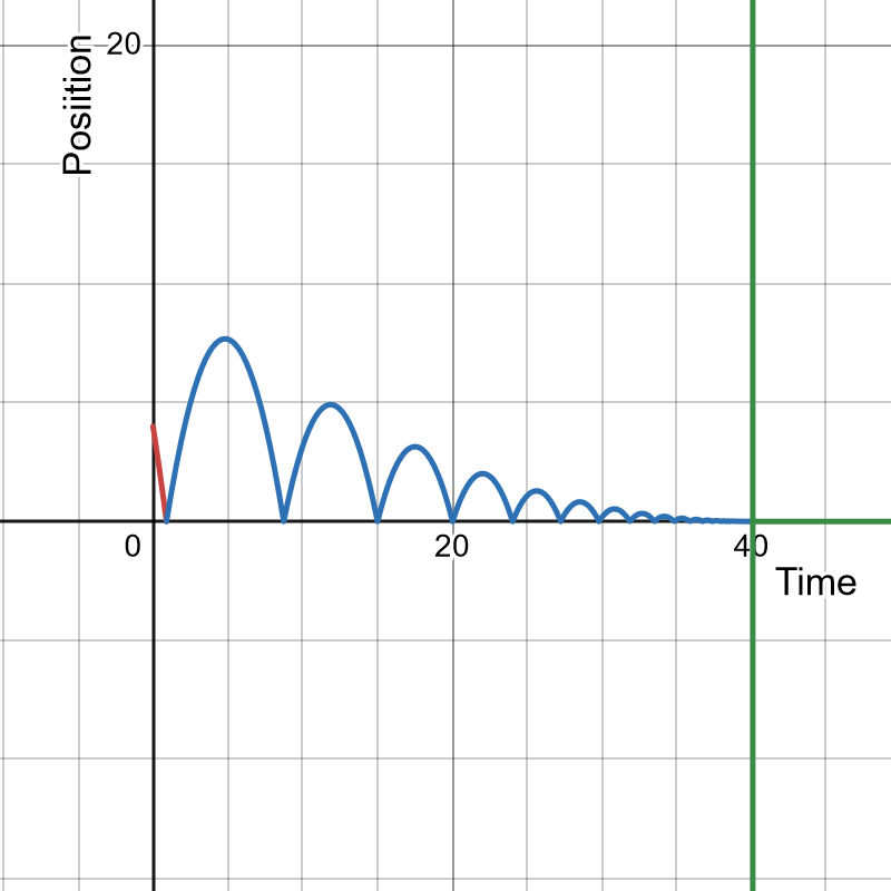
. When the ball hits the ground, it is instantaneously deflected upwards, resulting in its velocity being scaled by a factor of -R, where R is a constant strictly between 0 and 1 (the coefficient of restitution, or to put it in more ordinary terms, the “amount of bounciness”).

At what point does the ball stop bouncing?

The answer I expected was that the ball would never stop bouncing. I thought it would keep bouncing forever, with the bounces getting smaller and smaller in height, to a point where they were practically negligible, but I didn’t think there would be any definite point where it would stop altogether.

But it turns out that this is incorrect. While the ball does indeed bounce an infinite number of times, with the bounces getting smaller and smaller in height, that doesn’t mean it keeps bouncing forever. The bounces get smaller and smaller not only in height, but also in duration, and the sum of their durations converges to a finite limit, meaning there is a time T such that the sum of their durations is always less than, but can be made arbitrarily close to T. You can even calculate T using the following formula:

\displaystyle\label{time-bouncing-stops} T = t_1 - \frac {2 u_1} {g(1 - R)} \quad (1)

Here, t_1 is the time at which the first bounce begins and u_1 is the velocity of the ball at the start of this first bounce. (The formula does require you to know t_1 and u_1; it is possible to calculate t_1 and u_1 from the ball’s initial position and velocity, but the formula is a lot simpler and easier to understand if it’s left in terms of t_1 and u_1 rather than those initial values.)

Here’s how this formula can be derived. First, observe that between one bounce and the next, the ball moves with a constant acceleration g. Also, the ball’s position (or rather, the position of its bottom point) at the start of the bounce will be the position of the ground, which we’ll write as h. So if we consider a bounce starting at a time t_0, where the ball has velocity u_0 as it begins the bounce, the ball’s velocity v and position s at any subsequent time t before the next bounce will be given by the equations

\displaystyle \begin{aligned} v &= u_0 + g(t - t_0), \\ s &= h + u_0(t - t_0) + \frac {g(t - t_0)^2} 2. \end{aligned}

The next time the ball bounces, its position will be h again, so to find the time the current bounce ends and the next bounce begins, we should solve the equation s = h. Using the equation for s above, we can write s = h as an equivalent quadratic equation in t - t_0:

\displaystyle \frac {g(t - t_0)^2} 2 + u_0(t - t_0) = 0.

Since this equation has no constant term, it can be easily solved by factorising the LHS:

\displaystyle (t - t_0)\left( \frac {gt} 2 + u_0 \right) = 0

From this we see that s = h when t = t_0 (which we already knew) and also that s = h when

\displaystyle t = t_0 - \frac {2u_0} g.

This t is greater than t_0, since the ball moves away from the ground as it bounces, so the velocity u_0 at the start of the current bounce is nonzero and has the opposite sign to g. Hence we can interpret t as the time of the next bounce. Accordingly, the duration of the current bounce is t - t_0 = -2u_0/g. Furthermore, substituting t = t_0 - 2u_0/g into the equation for v gives us that the velocity at the end of the bounce is -u_0 (this is also obvious if you visualize the bounce as a parabola). Hence the velocity at the start of the next bounce will be Ru_0.

To summarize: if the ball has velocity u_0 at the start of a bounce, then the duration of the bounce will be -2u_0/g and the velocity of the start of the next bounce will be Ru_0.

If we now consider the full sequence of bounces, we have that the velocities at the start of each bounce are in a geometric progression. So we can give a general formula for the velocity u_n at the start of the nth bounce (for n \ge 1):

\displaystyle u_n = R^{n - 1} u_1.

Accordingly, the duration of the nth bounce will be -2 u_n/g = -2 R^{n - 1} u_1/g. Hence the total time taken by the first n bounces (not including any time before the first bounce) will be

\displaystyle \left( -\frac {2 u_1} g \right) + \left( -\frac {2 R u_1} g \right) + \dotsb + \left( -\frac {2 R^{n - 1} u_1} g \right),

This is a geometric series, which can also be written as

\displaystyle -\frac {2u_1(1 - R^n)} {g(1 - R)}.

Given that 0 < R < 1, we can take the limit as n approaches infinity, giving us the following expression for the total duration of the bounces:

\displaystyle -\frac {2u_1} {g(1 - R)}.

The t_1 term in (1) comes from the fact that there’s also some time before the first bounce.

What about t_1 and u_1? How do we calculate them? It’s not that much more complicated. We use the same quadratic equation as before, only now the ball’s initial position is not necessarily h, but some arbitrary r. If we say that the positive direction is upwards, then we can assume that h \le r, because the ball can’t be below the ground. We also have an arbitrary initial velocity u, and this doesn’t have to be positive like the velocity at the start of a bounce. It can be negative, positive or zero. So the equations of motion for the ball from time 0 up to the time the first bounce begins are:

\displaystyle \begin{aligned} v &= u + gt, \\ s &= r + ut + \frac {gt^2} 2. \end{aligned}

The equation s = h now comes out as the quadratic equation

\displaystyle \frac {gt^2} 2 + ut + r - h = 0.

The discriminant of this equation is

\displaystyle \Delta = u^2 - 2g(r - h).

Since h \le r and g 0 and g < 0, we have \tau_2 0, this means that \tau_1 \ge -2u/g > 0 and \tau_2 \le 0. If u < 0, this means that \tau_1 \ge 0 and \tau_2 \le -2u/g < 0. Whatever the case, we have that \tau_1 is non-negative and \tau_2 is non-positive. So we can interpret the two roots as endpoints of a “0th bounce” which is already in progress initially.

In particular, we have that the time the first bounce starts, t_1, is the time the 0th bounce ends, \tau_1. That is:

\displaystyle t_1 = -\frac {u + \sqrt \Delta} g = -\frac {u + \sqrt{u^2 - 2g(r - h)}} g.

As for u_1, we can substitute t = t_1 into the equation v = u + gt to get the velocity at the end of the 0th bounce: -\sqrt \Delta. The velocity at the start of the 1st bounce will be this scaled by -R, i.e.

\displaystyle u_1 = R \sqrt \Delta.

I started investigating this problem because I wanted to program a simulation of a ball bouncing on the ground. For this purpose, it would be ideal to have a function which, given a time t, tells you what the ball’s position will be. The derivations above already give us almost all the information we need to do this. The only missing thing is a way to determine what number bounce is in progress at time t. For every integer n, let

\displaystyle t_n = t_1 - \frac {2u_1(1 - R^{n - 1})} {g(1 - R)},

so that t_n is the time the nth bounce starts. Given a time t \ge t_1, we want to find the unique integer n such that t_n \le t < t_{n + 1}. Well, this chain of inequalities can also be written as

\displaystyle t_1 - \frac {2u_1(1 - R^{n - 1})} {g(1 - R)} \le t < t_1 - \frac {2u_1(1 - R^n)} {g(1 - R)}.

Doing some rearrangement, using the facts that -u_1/g and 1 - R are positive, we get the equivalent inequality

\displaystyle 1 - R^{n - 1} \le -\frac {g(t - t_1)(1 - R)} {2u_1} < 1 - R^n.

If we subtract each part of this chain of inequalities from 1, and then take its logarithm in base R, the order of the parts is preserved (because these two functions are both strictly decreasing, given that R < 1, and hence their composition is strictly increasing). So the chain of inequalities can also be written as

\displaystyle n - 1 \le \log_R \left( 1 + \frac {g(t - t_1)(1 - R)} {2u_1} \right) < n.

Now for each real number x, the “floor-plus-one” \lfloor x \rfloor + 1 of x is the unique integer n such that n - 1 \le x < n; hence we can conclude that

\displaystyle n = \left \lfloor \log_R \left( 1 + \frac {g(t - t_1)(1 - R)} {2u_1} \right) \right \rfloor + 1.

It is then straightforward to give a formula for s, using the fact that the nth bounce starts at time t_n, and the ball’s velocity as it begins this bounce is u_n.

\displaystyle s = h + u_n (t - t_n) + \frac {g(t - t_n)^2} 2.

Here’s a graph of the trajectory defined by this function, made in Desmos:

The vertical line is where the bouncing stops.

If you go to the Github Pages version of this article, you can also see what the simulation looks like (WordPress won’t let me put a video here). The code for it is on Github.

Implementing Python’s `cmp_to_key` function

Sorting functions in programming languages often take a parameter which allows the user to control how comparison is done when sorting. The most direct way to do this is to have the parameter be a comparison function, which takes two arguments and returns a value indicating how the first argument compares to the second argument.

For example, in Python, an implementation of insertion sort that allows the user to control how comparison is done might look like this:

import operator
from typing import Callable
def isort[T: Comparable](
    ls: list[T],
    cmp: Callable[[T, T], bool]=operator.lt
) -> None:
    for i, x in enumerate(ls[1:], start=1):
        j = i
        while j > 0 and not cmp(ls[j - 1], x):
            ls[j] = ls[j - 1]
            j -= 1
        ls[j] = x

However, Python’s built-in sorting functions work in a different way. Instead of taking a comparison function, they take a key function, which is a function of a single argument that may return anything. This function is used to generate a “key” for each object in the list to be sorted. The sorting is then based on comparison of those keys, rather than the underlying objects themselves, using the built-in comparison operator <. So to write a comparison function which is equivalent to the key function, we just apply the key function to the two arguments, and then compare the results using <. Here’s an implementation of a version of isort which uses a key function:

from typing import Protocol, Self
class Comparable(Protocol):
    def __lt__(self: Self, other: Self) -> bool:
        ...
def key_to_cmp[T, U: Comparable](
    key: Callable[[T], U]
) -> Callable[[T, T], bool]:
    return lambda x, y: key(x) < key(y)
def isort_by_key[T, U: Comparable](
    ls: list[T],
    key: Callable[[T], U]=lambda x: x
) -> None:
    return isort(ls, key_to_cmp(key))

Now, it’s easy to convert a key function to a comparison function: the key_to_cmp function here shows us to do it. But what about the reverse? How do we convert a comparison function to a key function? At least to me, it wasn’t totally obvious how to do this.

However, the solution is pretty simple once you realize that the return value from a key function can be absolutely anything, and that Python allows you to overload the < operator. So to do the conversion, we just need to define a new class, with < overloaded so that it uses the given comparison function when applied to instances of the class. The constructor for this class will then work as the function that does the conversion.

from dataclasses import dataclass
def cmp_to_key[T](
    cmp: Callable[[T, T], bool]
) -> Callable[[T], Comparable]:
    
    @dataclass(slots=True)
    class Key[T]:
        value: T
        def __lt__(self: Self, other: Self) -> bool:
            return cmp(self.value, other.value)
    return Key

Python actually provides a cmp_to_key function in the functools module which does just this.

The return type of this cmp_to_key function is an interesting one. Even though we know that the return class will be an instance of the locally-defined Key class, we haven’t indicated this in the return type. Indeed, we can’t do so because the Key class is defined within the scope of the cmp_to_key function, but the type declaration for cmp_to_key can only make use of names defined in the outer scope. And in fact, this is OK, because we shouldn’t be able to be any more specific about the return type. The Key class is an implementation detail, which callers of the cmp_to_key function have no need to be aware of. All callers need to know is that the function returned by cmp_to_key turns values of type T into comparable values, which is just what is conveyed by the Callable[[T], Comparable] type.

This way of typing cmp_to_key relies on subtyping—namely the fact that Comparable is a supertype of all the types Comparable[T] where T is another type. In a type system without subtyping, I think it might be possible to express the type using an existential type—something like this, in pseudo-Haskell syntax:

cmpToKey :: (a -> a -> Bool) -> exists b. Ord b => (a -> b)

This isn’t actually a legal Haskell type signature, because Haskell doesn’t allow you to express existential types directly; exists isn’t actually a Haskell keyword, though forall is. You’re supposed to express existential types by taking advantage of certain equivalences which allow you to express exists in terms of forall. I can’t figure out any way by which the type above could be expressed using forall, although given my level of fluency with this stuff, this is not a strong indicator that it’s impossible. Even if it is possible to express the type of cmpToKey in Haskell, I doubt it’s possible to actually implement it, because it would require a declaration of a type class instance within the function—something like this, which is definitely not valid Haskell syntax:

cmpToKey f =
    newtype Key a = Key a
    instance Ord (Key a) where
        Key x <= Key y = f x y
    
    Key

There’s probably something to be said here about the difference between type classes and classes in object-oriented programming, and the advantages and disadvantages of these two different approaches to polymorphism, but I don’t feel like I understand the subject well enough to say any more.

Enumerating the ordered k-partitions of an integer

Given two integers n and k, where k is non-negative, an ordered k-partition of n is a k-tuple (m_1, \dotsc, m_k) of positive integers such that

\displaystyle m_1 + \dotsb + m_k = n.

For example, the ordered 3-partitions of 5 are (1, 1, 3), (1, 2, 2), (1, 3, 1), (2, 1, 2), (2, 2, 1), and (3, 1, 1).

The problem I'm considering in this post is: how do you enumerate all the ordered k-partititions of n?

In the case where k = 0, the problem is simple. An ordered 0-partition is a 0-tuple. But there is only one 0-tuple: the empty tuple, (). And the sum of () is 0, which means the only integer () is an ordered 0-partition of is 0. So 0 has () as its only ordered 0-partition, while every other integer has no ordered 0-partitions.

In other cases, where k \ge 1, we can try to reduce the problem to instances of the problem where k is smaller, so that we can use recursion to arrive at a solution. Observe that an ordered k-partition of n will have the form (m_1, \dotsc, m_k), where m_1, …, m_k are positive integers that sum to n. Given that k \ge 1, we can talk about m_1 individually. By subtracting m_1 from both sides of the equation m_1 + \dotsb + m_k = n, we obtain the equivalent equation m_2 + \dotsb + m_k = n - m_1. This proves the following theorem:

Theorem. The ordered k-partitions of n are the k-tuples (m_1, \dotsc, m_k) of positive integers such that (m_2, \dotsc, m_k) is an ordered (k - 1)-partition of n - m_1.

This gives us a nice mathematical recursive characterization of the ordered k-partitions. If we write the set of all ordered k-partitions of n as P(n, k), and we denote concatenation of tuples by \frown, we can write the following equations:

\displaystyle \begin{aligned}     P(0, 0) &= \{ () \}, \\     P(n, 0) &= \varnothing &&\text{if } n \ne 0, \\     P(n, k) &= \bigcup_{m = 1}^\infty \{ (m) \frown t : t \in P(n - m, k - 1) \} &&\text{if } k \ge 1. \end{aligned}

However, these equations do not translate directly into a terminating algorithm, because of the union over all of the infinitely many positive integers m taken in the third equation.

But we don't necessarily need to examine all positive integers m, because for some of them, P(n - m, k - 1) may be empty, so that nothing is contributed to the overall union by this particular value of m. This suggests that we should consider the following sub-problem:

For which integers n and k, where k is non-negative, are there no ordered k-partitions of n?

This is easy to solve:

Theorem. For every integer n and every nonnegative integer k, the following statements are equivalent:

  • n has an ordered k-partition.
  • n = k = 0 or 1 \le k \le n.

Proof.

  • If n is negative, then it has no ordered k-partitions, because ordered k-partitions of n are tuples of positive integers that sum to n, but the sum of a tuple of positive integers is always non-negative.
  • If n < k, then n has no ordered k-partitions, because ordered k-partitions of n are tuples of k positive integers that sum to n, and the sum of k posiive integers cannot be less than k.
  • 0 has an ordered 0-partition, namely (). But no nonzero integer n has any ordered 0-partitions.
  • If 1 \le k \le n, then the ordered k-tuple consisting of k - 1 1s, followed by n - (k - 1) (which is positive since k - 1 < n), is an ordered k-partition of n.

\blacksquare

So, in the third equation above, the union only needs to be taken over values of m such that n - m = k - 1 = 0 (i.e. n = m and k = 1) or 1 \le k - 1 \le n - m (i.e. 2 \le k and m \le n - k + 1
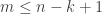
). Hence we can rewrite the equations as follows:

\displaystyle \begin{aligned}     P(0, 0) &= \{ () \}, \\     P(n, 0) &= \varnothing &&\text{if } n \ne 0, \\     P(n, 1) &= \varnothing &&\text{if } n \le 0, \\     P(n, 1) &= \{ (n) \} &&\text{if } n \ge 1, \\     P(n, k) &= \bigcup_{m = 1}^{n - k + 1} \{ (m) \frown t : t \in P(n - m, k - 1) \} &&\text{if } k \ge 2. \end{aligned}

This can now be translated straightforwardly to code in a programming language. For example, here's a Python implementation:

from typing import Iterator
def int_parts(n: int, k: int) -> Iterator[tuple[int, ...]]:
    if k == 0:
        if n == 0:
            yield ()
        return
    if k == 1:
        if n >= 1:
            yield (n,)
        return
    for m in range(1, n - k + 2):
        for p in int_parts(n - m, k - 1):
            yield (m,) + p

This is a pretty trivial subject, and I feel like my presentation of it here is somewhat incomplete (for example, I haven't said anything about how efficient the algorithm described here is). However, I think my standards for considering a post "complete" are a bit too high at the moment, as evidenced by the fact that I haven't made any posts on this blog for a couple of years, despite having written a number of unfinished drafts.

I think it would be good if whenever I learn something new, I would write down what I've learnt that very same day and make a blog post out of it, regardless of how trivial or in need of further exploration it might seem. So I'm going to attempt to do that from now on.

Dualities between depth-first search and breadth-first search

Something which I think is fairly well-known among programmers (I first learned it from reading Higher Order Perl) is that depth-first search and breadth-first search can be implemented in such a way that they differ only in their choice of data structure—depth-first search uses a stack (where you add to and remove from the same end), breadth-first search uses a queue (where you add to one end and remove from the other). Here is some illustrative Python code:

from collections import deque
from collections.abc import Iterable, Iterator
from typing import Protocol, TypeVar
T = TypeVar('T')
class Tree(Protocol[T]):
    def __call__(self, vertex: T) -> Iterable[T]:
        """Yield each of the vertex's children."""
def dfs(tree: Tree[T], start: T) -> Iterator[T]:
    stack = deque([start])
    
    while stack:
        vertex = stack.pop()
        yield vertex
        stack.extend(tree(vertex))
        
def bfs(tree: Tree[T], start: T) -> Iterator[T]:
    queue = deque([start])
    
    while queue:
        vertex = queue.pop()
        yield vertex
        queue.extendleft(tree(vertex))

Technical notes:

  • The Tree class is just an interface to say that a tree is a function (or another callable object) that, given something (a vertex), returns some other things of the same type (the children of the vertex).
  • Ordinary Python lists only support adding and removing elements efficiently (i.e. in constant time) at the back, because adding or removing elements at the front requires all the rest of the elements in the list to shift up or down by one place. They are therefore suitable for use as stacks, but not as queues. Instead I’ve used “deques” from the collections.deque module, which do support efficient adding and removing at both ends and hence make good queues as well as good stacks. Using an ordinary list for dfs would have been perfectly fine, but I’ve used deques for both functions just to makes the code more symmetric.

It’s worth noting however that there is a slight difference between how these two functions work, in that dfs yields sibling vertices in reverse order, compared to bfs (or to the order within the tree itself): for example, list(dfs(lambda _: (1, 2), 0)) evaluates to [0, 2, 1] while list(bfs(lambda _: (1, 2), 0)) evaluates to [0, 1, 2]. This isn’t an inherent consequence of the depth-first-ness or breadth-first-ness of the search order; it’s just due to the fact that with a stack, you take things out in the reverse order compared to how you put them in.

One way to rectify this while preserving the stack/queue duality is to keep vertices themselves out of the stack/queue. Instead, we can directly store the iterators over child vertices that we get from the tree:

def dfs(tree: Tree[T], start: T) -> Iterator[T]:
    stack = deque([iter([start])])
    
    while stack:
        try:
            vertex = next(stack[-1])
        except StopIteration:
            del stack[-1]
        else:
            yield vertex
            stack.append(iter(tree(vertex)))
def bfs(tree: Tree[T], start: T) -> Iterator[T]:
    queue = deque([iter([start])])
    
    while queue:
        try:
            vertex = next(queue[-1])
        except StopIteration:
            del queue[-1]
        else:
            yield vertex
            queue.appendleft(iter(tree(vertex)))

For dfs, this approach is likely to improve memory usage as well, since it means that only one iterator needs to be stored for each ancestor of the vertex currently being searched, while with the old dfs function, each younger sibling of each ancestor needs to be stored (and while it is possible for there to be no younger siblings, in which case the old implementation saves more memory, it is more likely that there will be many younger siblings in practice).

For bfs, on the other hand, there is actually only a tiny improvement in memory usage: it will still use the same amount of memory, it will just take a bit longer to get to that point. To be more precise, note that we can divide a tree into “levels”, where the first level consists of the root alone, the second level consists of the root’s children, the third level consists of the root’s grandchildren (i.e. all the children of vertices on the first level), etc. The distinctive characteristic of a breadth-first search is that it always completes one level before it moves on to the next. We can call vertices on the same level “cousins”. Also, given a bunch of cousin vertices, which we can think of as a “part” of the level they’re on, we can say that the part of the previous level consisting of the parents of those cousins is immediately “above”, and the part of the next level consisting of the children of those cousins is immediately “below”.

Now, suppose we’re doing a breadth-first search, and a vertex v at level n is currently being searched. The queue will contain the remaining vertices on level n (i.e. v‘s younger cousins), and the vertices on level n + 1 that have already been added from searching older cousins of v (i.e. the children of those older cousins). In the original bfs function these vertices are actually there in the queue, so the size S of the queue is the size of the remaining part of level n (= the number of younger cousins v has), plus the size of the part of level n + 1 that’s below the reached part of level n (= the total number of children v‘s older cousins have). In iterator-based bfs, on the other hand, the vertices are packaged into iterators according to their common parents; so the size of the queue is the size of the part of level n – 1 that’s above the remaining part of level n, plus the size of the reached part of level n. If the levels are increasing in size, this will generally be a smaller size than S. But at some point later on in the search, we’ll get to the children of v on level n + 1. Then, the size of the queue will be the size of the part of level n that’s above the remaining part of level n + 1, plus the size of the reached part of level n + 1. But the vertices remaining at this point are just the younger cousins of v‘s children, so the part of level n above them consists of v‘s younger cousins. Likewise the reached part of level n + 1 at this point consists of the children of v‘s older cousins. In other words the queue is the same size as it would have been for the original bfs function when searching v.

(There are better ways of doing a memory-efficient breadth-first search, which we’ll say more about shortly.)

Anyway, an alternative way of making dfs yield sibling vertices in the right order would be to write it recursively. This amounts to doing exactly the same thing as using a stack of iterators, except that rather than using an explicit stack we use the language’s call stack, and rather than explicitly working with iterators we use a for loop.

def dfs(tree: Tree[T], start: T) -> Iterator[T]:
    yield start
    
    for vertex in tree(start):
        yield from dfs(tree, vertex)

This is definitely the shortest and clearest way to write a depth-first search. Its main drawback is that in a language like Python you might end up running into a recursion limit, although it would have to be a very large and deep tree to get to that point.

And although it’s not really a meaningful drawback, the connection with breadth-first search seems to be lost by writing dfs recursively like this. Obviously one can’t write a breadth-first search recursively in the same way as a straightforward translation of iterator-based bfs, since recursion necessarily uses an implicit stack rather than an implicit queue.

However, quite surprisingly, it turns out that there is still a simple alteration we can make in order to make this recursive dfs function do a breadth-first search instead. This is clearest in Haskell notation, where it amounts to reversing the order of a Kleisli composition:

import Control.Monad
data Tree a = Tree a [Tree a]
children :: Tree a -> [Tree a]
children (Tree u vs) = vs
dfs :: Tree a -> [Tree a]
dfs t = [t] ++ (children >=> dfs) t
bfs :: Tree a -> [Tree a]
bfs t = [t] ++ (bfs >=> children) t

In Python, that new bfs function would look like this:

def bfs(tree: Tree[T], start: T) -> Iterator[T]:
    yield start
    
    for vertex in bfs(tree, start):
        yield from tree(vertex)

Basically we’ve exchanged the places of the call to tree and the recursive call to the search function.

While this is a very short way to write a breadth-first search, I would say it is rather more difficult to understand, compared to recursive dfs. This is mainly due to the fact that, unlike recursive dfs (which could easily be rewritten to return a sequence, rather than just an iterator) it makes essential use of the fact that it’s a generator function, so that the recursive calls in it don’t simply nest, but are rather interwoven with each other. The best way to understand how it works is to insert some logging and see it in action.

from functools import partial
from operator import getitem
import itertools as it
    
def bfs(tree: Tree[T], start: T) -> Iterator[T]:
    call_counter = it.count()
    def _bfs() -> Iterator[T]:
        call_id = next(call_counter)
        print(f'call ID {call_id} begun')
        print(f'call ID {call_id}: yielding {start}')
        yield start
        
        for vertex in _bfs():
            print(f'call ID {call_id}: yielding children of {vertex}')
        
            for child in tree(vertex):
                print(f'call ID {call_id}: yielding {child}')
                yield child
            
    yield from _bfs()
>>> tree = {1: (2, 3), 2: (4,), 3: (5, 6), 4: (7,), 5: (), 6: (8,), 7: (), 8: ()}
>>> search = bfs(partial(getitem, tree), 1)
>>> list(it.islice(search, 8))
call ID 0 begun
call ID 0: yielding 1
call ID 1 begun
call ID 1: yielding 1
call ID 0: yielding children of 1
call ID 0: yielding 2
call ID 0: yielding 3
call ID 2 begun
call ID 2: yielding 1
call ID 1: yielding children of 1
call ID 1: yielding 2
call ID 0: yielding children of 2
call ID 0: yielding 4
call ID 1: yielding 3
call ID 0: yielding children of 3
call ID 0: yielding 5
call ID 0: yielding 6
call ID 3 begun
call ID 3: yielding 1
call ID 2: yielding children of 1
call ID 2: yielding 2
call ID 1: yielding children of 2
call ID 1: yielding 4
call ID 0: yielding children of 4
call ID 0: yielding 7
call ID 2: yielding 3
call ID 1: yielding children of 3
call ID 1: yielding 5
call ID 0: yielding children of 5
call ID 1: yielding 6
call ID 0: yielding children of 6
call ID 0: yielding 8
[1, 2, 3, 4, 5, 6, 7, 8]
>>> next(search)
call ID 4 begun
call ID 4: yielding 1
call ID 3: yielding children of 1
call ID 3: yielding 2
call ID 2: yielding children of 2
call ID 2: yielding 4
call ID 1: yielding children of 4
call ID 1: yielding 7
call ID 0: yielding children of 7
call ID 3: yielding 3
call ID 2: yielding children of 3
call ID 2: yielding 5
call ID 1: yielding children of 5
call ID 2: yielding 6
call ID 1: yielding children of 6
call ID 1: yielding 8
call ID 0: yielding children of 8
call ID 5 begun
call ID 5: yielding 1
call ID 4: yielding children of 1
call ID 4: yielding 2
call ID 3: yielding children of 2
call ID 3: yielding 4
call ID 2: yielding children of 4
call ID 2: yielding 7
call ID 1: yielding children of 7
call ID 4: yielding 3
call ID 3: yielding children of 3
call ID 3: yielding 5
call ID 2: yielding children of 5
call ID 3: yielding 6
call ID 2: yielding children of 6
call ID 2: yielding 8
call ID 1: yielding children of 8
call ID 6 begun
...

Note that although it does yield the vertices in the correct, breadth-first order, it also gets itself into an infinite loop once it’s done, rather than just terminating! So in that respect, its behaviour is not quite simply that of recursive dfs plus doing the search in breadth-first order.

Let’s forget for a moment about the fact that only the yields from call ID 0 are actually sent back to the original caller, and just look at the sequence of nodes that are yielded, regardless of which recursive sub-call does the yielding. We’ll also break this sequence into segments, with a new segment starting whenever a new begins.

1
1, 2, 3
1, 2, 4, 3, 5, 6
1, 2, 4, 7, 3, 5, 6, 8

Do you see the pattern?

  • In each segment, the vertices yielded are all those up to a certain level in the tree. At first we only see 1, the unique vertex at the first level; in each subsequent segment the maximum reachable level increases by 1.
  • Within a segment, all vertices within the reachable levels are yielded in depth-first order. (But only the ones from the newest reachable level end up reaching the original caller, since those are the ones yielded by call ID 0).

So what this bfs function is actually doing is really something called iterative deepening depth-first search. It simply does a depth-first search, but only to a limited depth. Initially it only goes to the first level, but whenever it finishes searching, it starts again while increasing the depth limit by one. And it only yields the new vertices on the most recently-reached level. The effect of this is to yield vertices in breadth-first order, so in terms of the result it’s a breadth-first search, but in terms of the algorithm itself it’s more like a variation on depth-first search. It also now makes sense why it gets into an infinite loop eventually: after a certain point any deeper level contains no more vertices, but the algorithm will keep repeating the depth-first search and searching the new empty level.

This might seem like quite a silly way to do things, and it certainly involves a lot of redundant work compared to the alternative, since the higher levels of the tree are searched repeatedly again and again. However, it does have a big advantage in terms of memory usage, because, since it’s really a depth-first search, it has the memory usage of a depth-first search: it only needs to store the ancestors of the vertex currently being searched; in short, its memory usage corresponds to the depth of the tree. With a queue-based breadth-first search, on the other hand, the size of the queue is basically proportional to the size of the level currently being searched, i.e. the tree’s breadth. And trees in practice tend to be broader than they are deep. In fact they are often exponentially broader than they are deep, since all it takes for that to be the case is for the average number of children per vertex (the “branching factor”) to be greater than 1. In such a situation, the redundant work from searching higher levels repeatedly is less of an issue, since the deepest level reached accounts for the majority of the work in searching the tree anyway.

Iterative deepening depth-first search is known as IDDFS for short, and it’s generally associated with the field of artificial intelligence, since that’s where people are (or were) most likely to deal with problems involving brute-force search of massive trees with high branching factors, such as deciding the next move to play in a game of chess; this involves considering each of the possible moves, and for each move, the possible moves that could be made afterwards, and for each of the resulting 2-move sequences, the third moves that could be made afterwards; so it can naturally be modelled as a big tree. Although, nowadays, with the field being more focussed on machine learning, people might not be directly programming these kinds of tree searches so often any more (though I’m just guessing here—I don’t know that much about AI).

I’m not sure how well-known it is that you can write IDDFS as the simple recursive function above. You can of course write it in a more “direct” manner, and this is how it’s presented in standard references such as Korf (1985) or Russell & Norvig (2010). I learned about the connection between the recursive bfs implementation and IDDFS from a comment on an ActiveState code recipe by David Eppstein (and I learned about the recursive bfs implementation in the first place from a StackOverflow answer by Herrington Darkholme, who, it turns out, got it originally from the same code recipe as mentioned on this blog post of theirs).

For the record, here’s a more direct IDDFS implementation, including a termination check so that it stops once it reaches a level where there are no vertices:

import itertools as it
def depth_labelled(tree: Tree[T], start: T) -> tuple[Tree[tuple[T, int]], tuple[T, int]]:
    def new_tree(vertex_with_depth: tuple[T, int]) -> Iterator[tuple[T, int]]:
        vertex, depth = vertex_with_depth
        
        for child in tree(vertex):
            yield (child, depth + 1)
    return new_tree, (start, 0)
def depth_limited(tree: Tree[T], start: T, limit: int) -> tuple[Tree[tuple[T, int]], tuple[T, int]]:
    tree, start = depth_labelled(tree, start)
    
    def new_tree(vertex_with_depth: tuple[T, int]) -> Iterator[tuple[T, int]]:
        vertex, depth = vertex_with_depth
        if depth < limit:
            yield from tree(vertex_with_depth)
    return new_tree, start
def iddfs(tree: Tree[T], start: T) -> Iterator[T]:
    for limit in it.count():
        limited_tree = depth_limited(tree, start, limit)
        level_size = 0
        for vertex, depth in dfs(*limited_tree):
            if depth == limit:
                yield vertex
                level_size += 1
        if not level_size:
            break

To adapt the termination check to the original recursive bfs function, we have to modify the logic a bit so that we only get one level at a time:

def bfs(tree: Tree[T], start: T) -> Iterator[T]:
    yield start
    iterator = bfs(tree, start)
    level_size = 1
    
    while level_size:
        level = it.islice(iterator, level_size)
        level_size = 0
    
        for vertex in level:
            for child in tree(vertex):
                yield child
                level_size += 1

The function is now behaviorally more of an exact counterpart of dfs, although it is no longer so similar in implementation.

I still find it to be a bit of a startling coincidence that just switching the order of those two calls within the recursive implementation of dfs makes it into a breadth-first search (even if it behaves somewhat differently with regard to termination). It seems like something there should be a deeper explanation for, but I don’t know what it would be. And does it have anything to do with the stack/queue duality? The way IDDFS works doesn’t seem to involve a queue, not even implicitly, so maybe not. I don’t have answers to these questions, unfortunately.


Code snippets from this article are available on GitHub.

A simple motivation for the notion of a natural transformation

A natural transformation is an operation on a category, or more precisely a family of operations, one for each object in the category, which is preserved by morphisms in the category.

Each operation in the family is associated with a specific object A in the category, which it is said to be on. The operation itself is an endomorphism on A, modulo application of functors in a regular way to the domain and codomain. That is, it is a morphism from F(A) to G(A) for some functors F and G which are the same for every object. We call F and G the domain and codomain of the operation, respectively.

For example, multiplication in a group G is a function from U(G)^2 to U, where U is the forgetful functor from groups to sets. So the domain and codomain of the natural transformation corresponding to multiplication in groups are FU and U respectively, where F is the endofunctor on the category of sets such that for every set A, we have F(A) = A^2, and for every function f : A \to B and any two elements x and y of A^2, we have F(f)(x, y) = (f(x), f(y)).

If, for every object A, we write the operation on A as \alpha_A, then the naturality condition requires that for every morphism f : A \to B, we have G(f) \circ \alpha_A = \alpha_B \circ F(f). This is just the requirement that f “preserves” the operation: applying f to the output is the same as using the value under f as the input (modulo the functors we need to get the types right).

Consider the example of groups: a group homomorphism f : G \to H needs to have the property that for any two elements x and y of U(G), we have U(f)(xy) = U(f)(x) U(f)(y). (Of course we don’t usually write the forgetful functor explicitly, but we’re trying to be precise here.) If we write multiplication in G and H using prefix symbols \alpha_G and \alpha_H respectively, then this equation becomes U(f)(\alpha_G(x, y)) = \alpha_H(U(f)(x), U(f)(y)). Looking at the way F acts on morphisms, we see that this can be further rewritten as

\displaystyle U(f)(\alpha_G(x, y)) = \alpha_H(F(U(f))(x, y)),

i.e.

\displaystyle U(f) \circ \alpha_G = \alpha_H \circ F(U(f)).

I like this way of motivating natural transformations because—well, first of all because it’s a way of motivating natural transformations at all, which is more than pretty much every category theory introduction I’ve seen does, at least if you don’t count saying that there ought to be some notion of morphism between functors, and then declaring by fiat that natural transformations are the appropriate notion of morphism between functors, as motivation. But also because it allows us to reconcile the formal category-theoretic understanding of a category as having its morphisms as part of its data with the perhaps more natural pre-formal understanding of a category as having operations as part of its data, and morphisms being characterized by their preservation of those operations.

In general, we can say that an operation on a category X is a family of morphisms \alpha_A : F(A) \to G(A) on objects A of X, where F and G are functors from X to some other category Y. In other words, it is like a natural transformation but it doesn’t need to satisfy the naturality condition. Now, if we have an operation like this we can consider the set of the morphisms f : A \to B in X which do satisfy the natural condition, i.e. have G(f) \alpha_A = \alpha_B F(f). It turns out that this set of morphisms is always closed under composition and contains every identity morphism, and therefore induces a subcategory of X:

Proof that it’s closed under composition. Suppose f : A \to B and g : B \to C are morphisms in X and G(f) \alpha_A = \alpha_B F(f) and G(g) \alpha_B = \alpha_C F(g). Then

\displaystyle G(gf) \alpha_A = G(g) G(f) \alpha_A = G(g) \alpha_B F(f) = \alpha_C F(g) F(f) = \alpha_C F(gf).

Proof that it contains every identity morphism. Suppose A is an object in X. Then

\displaystyle G(1_A) \alpha_A = 1_{G(A)} \alpha_A = \alpha_A = \alpha_A 1_{F(A)} = \alpha_A F(1_A).

For example, if we consider the category of groups and functions between groups, the category of groups and group homomorphisms is induced in this way as a subcategory by the operation of multiplication in groups.

It’s interesting to consider the converse: given a category X and a subcategory Y of X, under what circumstances is there is a category Z, functors F and G from X to Z, and an operation \alpha : F \to G such that the morphisms in X are precisely the morphisms f : A \to B in X with G(f) \circ \alpha_A = \alpha_B \circ F(f)? Obviously Z will have to still contain every object in X (since the construction described here only limits the morphisms in the subcategory, not the objects), but I will leave any more detailed consideration of this question for readers.

Notes on periodic functions

A period of a function f : ℝ → X is a T ∈ ℝ such that for every t ∈ ℝ, we have f(t + T) = f(t). Note that X may be any set; the definition does not refer to any structure on X other than its equality relation.

For every function f : ℝ → X, the set of periods of f is an additive subgroup of :

  • For any two periods T1 and T2 of f and every t ∈ ℝ, we have
    f(t + T1 + T2) = f(t + T1) = f(t),
    so T1 + T2 is a period of f.
  • For every period T of f and every t ∈ ℝ, we have
    f(t − T) = f((t − T) + T) = f(t),
    so  − T is a period of f.

Therefore, we call it the group of periods of f.

The converse also holds: every additive subgroup G of is the group of periods of a function, namely the canonical projection f : ℝ → ℝ/G (which takes every t ∈ ℝ to its equivalence class wrt the equivalence relation {(t1, t2) : t2 − t1 ∈ G}):

  • For every T ∈ G and every t ∈ ℝ, we have (t + T) − t = T ∈ G and hence f(t + T) = f(t), so T is a period of f.
  • Conversely, for every period T of f, we have f(T) = f(0) and hence T − 0 = T ∈ G.

Henceforth, we shall always refer to additive subgroups of as groups of periods.

It is worth noting explicitly that, in addition to the two closure properties proven above, the fact that the groups of periods are groups implies that they are closed under integer multiples, and in particular contain 0.

A function is aperiodic iff its group of periods is trivial, i.e. 0 is its only period. Otherwise, it is periodic.

If a group G of periods is nontrivial and cyclic, then it has a nonzero generator a. Since the set of the generators of G is closed under negation, we can choose a to be positive. This a is then the least positive element of G, because for every positive x ∈ G, there is an n ∈ ℤ such that x = na where n ∈ ℤ, and this n has to be positive (since x and a are positive), so that x ≥ a. The logic here works for any ordered group, not just groups of periods. It also works for any positive generator of G—so the least positive element of G is the only positive generator of G.

Conversely, if a group G of periods has a least positive element a, then a generates G. To see this, suppose x ∈ G and let n be the floor of x/a, so that n ≤ x/a < n + 1, i.e. na ≤ x < (n + 1)a, i.e. 0 ≤ x − na < a. Then x − na is an element of G less than a, so it cannot be positive; it must be 0, so that x = na. (The logic here doesn’t work for any ordered group, because it relies on the Archimedean property of the real numbers.)

So a nontrivial group G of periods has a least positive element a iff it is cyclic, in which case a is the unique positive generator of G. In this situation, we call a the fundamental period of G, or more loosely just the period of G.

The “canonical” examples of periodic functions have fundamental periods. For example, the sine and cosine functions have a fundamental period of 2π. However, constant functions are also technically periodic, and they do not have fundamental periods: a function f : ℝ → X is constant iff its group of periods is . There are more obscure examples. Consider the indicator function 1 of . For every T ∈ ℚ and every t ∈ ℝ, we have t + T ∈ ℚ iff t ∈ ℚ and hence f(t + T) = f(t); so T is a period of f. On the other hand, for every irrational T ∈ ℝ, we have ( − T) + T = 0 ∈ ℚ but  − T ∉ ℚ, and hence f(( − T) + T) = 1 but f( − T) = 0; so there is a t ∈ ℝ such that f(t + T) ≠ f(t), and hence T is not a period of f. It follows that the group of periods of 1 is .

There is a topological criterion which can be used to determine whether a periodic function has a fundamental period: a group G of periods is cyclic iff it is not dense in . To see this, observe first that if G is dense in , then it has elements arbitrarily close to 0, symmetrically on both the positive and negative sides of the number line (since G is closed under negation). Therefore G does not have a least positive element and hence is acyclic.

Conversely, suppose G is acyclic and hence has no least positive element. Then for every positive x ∈ G, there is a positive y ∈ G less than x. The difference x − y is also a positive element of G less than x, and at least one of y and x − y is less than or equal to x/2 (otherwise their sum would be greater than x). So in fact there is a positive y ∈ G less than or equal to x/2. By repeatedly applying this we can see that for every n ∈ ℕ, there is a positive y ∈ G less than or equal to x/2n. So G has positive elements arbitrarily close to 0. It follows that for every a ∈ ℝ and every positive ε ∈ ℝ, there is a positive x ∈ G less than ε. The interval (a − ε, a + ε), being of length 2ε > x, must contain nx for some n ∈ ℤ. And since G is closed under integer multiples, we have nx ∈ G. So G has elements arbitrarily close to a. This holds for every a ∈ ℝ, so G is dense in .

This criterion is simplified for continuous periodic functions f : ℝ → X, where X is an accessible topological space (a topological space X is accessible iff any two distinct points in X have neighbourhoods not containing the other point). This is because the group G of periods of such a function f is closed. To see this, suppose T0 is a limit point of G; it will suffice to prove that T0 ∈ G. To see that, suppose t ∈ ℝ; it will suffice to prove that f(t + T0) = f(t). To see that, suppose N is a neighbourhood of f(t + T0); it will suffice to prove that f(t) ∈ N. Since f is continuous, so is its right-composition with adding t. Therefore there is a neighbourhood M of T0 such that f(t + M) ⊆ N. And since T0 is a limit point of G, there is a T ∈ M ∩ G. Since T ∈ M, we have f(t + T) ∈ N. Since T ∈ G, we have f(t + T) = f(t) and hence f(t) ∈ N.

Since G is closed, it is equal to its closure. So it can only be dense in (i.e. have its closure equal to ) iff it is equal to . Therefore, given that f is a continuous periodic function with an accessible codomain, it has a fundamental period iff it is nonconstant.


A proof of the boundedness theorem by induction

As usual, this post can be viewed as a PDF.

Theorem (Boundedness Theorem). A continuous real-valued function on a closed interval is bounded.

Proof. Suppose f is such a function and [a, b] is its domain. First, observe that for every c ∈ [a, b], since f is continuous at c, there is a positive \delta \in {\mathbb R} such that for every x ∈ [a, b]∩(c − δ, c + δ), we have f(x)∈(f(c)−1, f(c)+1). So there is a neighbourhood of c, namely (c − δ, c +  δ), on which f is bounded. Thus f is, in a sense, locally bounded at every point in its domain; the problem is to prove that this local boundedness implies global boundedness.

In textbook proofs of the boundedness theorem, this is generally done using what I would regard as a trick, such as supposing f isn’t bounded and using the Bolzano-Weierstrass theorem to obtain a contradiction. More advanced texts may appeal to the compactness of [a, b], but the proof that [a, b] is compact (the Heine-Borel theorem) amounts to basically the same logic, and is usually no less trickful1.

However, if we think about how to construct an algorithm to find a global bound (often a helpful move to make—the un-situated-in-time-ness of ordinary mathematical language can be quite thought-limiting) then there is a procedure which, in my opinion, is quite obvious and immediately suggests itself. Just start on the left, with the singleton interval {a}, on which f is certainly bounded, and repeatedly apply local boundedness to the right endpoint, gradually expanding the subinterval of [a, b] on which we know f to be bounded. At each step the existing subinterval has a bound, and the neighbourhood of the right endpoint has a bound; taking the maximum of these two bounds gives us a bound of the whole expanded subinterval formed by unioning2 the neighbourhood with the existing subinterval. Eventually the right endpoint will reach b and we will no longer be able to expand it further, at which point we stop and observe that we have bounded the whole of [a, b]. (Sanity check: why would this fail for (a, b)? Because then we wouldn’t be able to take the right endpoint to b; there would be nowhere to stop the procedure, without leaving a part of the right of (a, b) unbounded.)

Of course, this algorithm will not in general terminate in a finite number of steps, but this is no issue; don’t let your thinking be limited by the arbitrary limitations of physical machines. Obviously, it is still necessary to prove that this algorithm will terminate, even if it takes infinitely many steps. Since we’re now dealing with the distinctions among the infinite quantities, we’re going to need to use some set-theoretic machinery (which is why you won’t see this proof in introductory real analysis textbooks). I’ll assume that you are familiar with the ordinals, the techniques of transfinite induction and recursion, and Burali-Forti’s paradox (which says that there is no set of all ordinals).

Here’s the plan. Using transfinite recursion, we shall construct an ordinal-indexed sequence xα of members of [a, b] such that every ordinal α has the following properties:

  1. The function f is bounded on [a, xα].

  2. We have xα ≤ xα + 1, and if xα = xα + 1, then xα + 1 = b.

Then, since there are a proper class’s worth of ordinals and [a, b] is just a set, the sequence xα will have to repeat3, so there will be ordinals α and β such that α < β and xα = xβ. By (2), the sequence xα will be nondecreasing, so we will have xα ≤ xα + 1 ≤ xβ and hence xα = xα + 1 = xβ = b. Then by (1), it will follow that f is bounded on [a, b].

All we need to do to complete the proof is describe the recursion and make it clear that it is a valid recursion (i.e. all of the assumed properties used to construct the next term of the sequence are preserved by the constructed sequence with the next term added).

Base case
Let x0 = a and observe that f is bounded on {a} by |f(a)|.
Successor case
For every ordinal α, if we assume that xα ∈ [a, b], then since f is continuous, there is a positive \delta \in {\mathbb R} such that f is bounded on [xα, xα + δ] by some M. Let xα + 1 = min(b, xα + δ), and observe that:

  • If b ≤ xα + δ, then xα + 1 = b and hence a ≤ xα ≤ xα + 1 ≤ b. Otherwise, we have xα + 1 = xα + δ and hence a ≤ xα < xα + 1 ≤ b, with the middle inequality strict, so that we can only have xα = xα + 1 when xα + 1 = b.
  • We have xα + 1 ≤ xα + δ, so f is bounded by M on [xα, xα + 1] as well as [xα, xα + δ]. Assuming f is bounded on [a, xα] by some L, it follows that f is bounded on [a, xα + 1] by max(L, M).

Limit case

For every limit ordinal λ, let A = {xα : α < λ}. Then A contains x0 and hence is nonempty, and is bounded above by b, so it has a supremum. Let xλ = supA, and observe that:

  • If we assume that A ⊆ [a, b], then since A is nonempty and xλ is ge every member of A, we have xλ ≥ a; and since b bounds A above and xλ is the smallest upper bound of A, we also have xλ ≤ b.
  • Since xλ ∈ [a, b] and f is continuous, there is a positive \delta \in {\mathbb R} such that f is bounded on [xλ − δ, xλ] by some M. And since xλ = supA, there is an ordinal α < λ such that xλ − δ < xα and hence f is bounded on [xα, xλ] by M. Assuming f is bounded on [a, xα] by some L, it follows that f is bounded on [a, xλ] by max(L, M).

And that’s it.

Of course, this proof is a bit tedious. There might be ways to make it shorter (maybe we can use Zorn’s lemma instead of transfinite induction). But the advantage it has over other proofs of the boundedness theorem I’ve seen is that it falls out more or less automatically, without requiring any flashes of insight.


  1. This word doesn’t appear to exist currently, but it needs inventing.

  2. Another word that needs inventing. OK, I could use “uniting”, but I suspect people wouldn’t immediately make the connection with the union operation on sets if I used that word.

  3. This is a sort of infinitary pigeonhole principle.

Notes on proving the completeness theorem for propositional logic

NB: I’ve opted to just get straight to the point with this post rather than attempting to introduce the subject first, so it may be of little interest to readers who aren’t already interested in proving the completeness theorem for propositional logic.

A PDF version of this document is available here.

The key thing I had to realize for the proof of the completeness theorem for propositional logic to “make sense” to me was that interpretations of a language of propositional logic can be thought of as theories.

Normally, an interpretation of a language L of propositional logic is thought of as a function υ from the set of the sentence variables in L to {0, 1}, which is extended to the set of the formulas in L by letting υ(⊥)=0 and recursively letting
\upsilon(\phi \rightarrow \psi) = \upsilon(\psi)^{\upsilon(\phi)} = \begin{cases}         0 &\quad \text{if } \upsilon(\phi) = 0 \text{ or } \upsilon(\psi) = 1, \\         1 &\quad \text{if } \upsilon(\phi) = 1 \text{ and } \upsilon(\psi) = 0     \end{cases}
for every pair of sentences ϕ and ψ in L (assuming and are the primitive connectives). The value under υ of a sentence ϕ is thought of as the truth value of ϕ under υ, with 0 standing for falsity and 1 standing for truth.

A theory in L, on the other hand, is thought of as a set of sentences in L, these sentences being the nonlogical axioms of the theory. It’s a completely different type of object from an interpretation.

But if you think about what these formal concepts are trying to get at, they’re quite similar. Both of them are essentially requirements that certain sentences be true. A theory requires its nonlogical axioms to be true. An interpretation requires the sentences true under it to be true, and the sentences false under it to be false, which might appear to be a slightly more elaborate concept, but since a sentence is false iff its negation is true, you know what sentences an interpretation makes false if you know what sentences it makes true. The only substantial difference is that an interpretation is subject to certain restrictions compared to a general theory:

  1. An interpretation of L must require every sentence variable in L to be either true or false (and not both).

  2. An interpretation of L must require to be false.

  3. For every pair of sentences ϕ and ψ in L, an interpretation of L must require ϕ → ψ to be true iff it requires ϕ to be false or requires ψ to be true (or both).

Formally, we can define a function f on the set of the interpretations of L by the rule that for every interpretation υ of L, we have
f(\upsilon) = \{\phi : \upsilon(\phi) = 1\} \cup \{\neg \phi : \upsilon(\phi) = 0\}.
This function f is an injection into the set of the theories in L. But it is not surjective—for every theory M in L, the value f−1(M) exists only if the statements below hold:

  1. For every sentence variable A in L, exactly one of A and ¬A is a member of M.
  2. ⊥ ∉ M.

  3. For every pair of sentences ϕ and ψ in L, we have ϕ → ψ ∈ M iff ϕ ∉ M or ψ ∈ M.

An interpretation could reasonably be defined as a theory M in L with properties (1)-(3) above.

Now, the completeness theorem says that every syntactically consistent theory in L is semantically consistent, i.e. has a model. A model of a theory T in L is an interpretation of L under which every member of T is true, so if we adopt the definition of interpretations as theories, we can say that a model of T is an extension of T which is an interpretation of L. This leads us to the idea that in order to construct a model of an arbitrary syntactically consistent theory T in L, we will have to extend T by adding new members.

But how exactly do we extend T? Here, it helps to recall the soundness theorem, which is the converse of completeness: it says that every semantically consistent theory in L is syntactically consistent. (This is generally straightforward to prove from the definition of syntactic consequence. I’m not going to prove it here because I’m trying to be agnostic about exactly how syntactic consequences are defined, and the proof is different depending on how syntactic consequences are defined.) Every interpretation of L, thought of as a theory in L, is certainly semantically consistent (since it has itself as an extension) and hence, by soundness, syntactically consistent. Therefore one thing we definitely need to do as we add new members to T, in order for it to eventually become an interpretation of L, is preserve the syntactic consistency of T.

In fact, it’s not too difficult to see that every theory M in L which can be thought of as an interpretation of L is not only syntactically consistent, but maximally syntactically consistent: every proper extension of M is syntactically inconsistent.

To see this, first, observe that for every sentence ϕ in L, since ¬ϕ abbreviates ϕ → ⊥, property (3) tells us that ¬ϕ ∈ M iff ϕ ∉ M or ⊥ ∈ M; and M never contains . So we have ¬ϕ ∈ M iff ϕ ∉ M. In other words, M contains exactly one of ϕ and ¬ϕ.

Now, suppose M is a proper extension of M. Then it has a member ϕ which is not a member of M. The negation of ϕ must then be a member of M. Since M extends M, it follows that ¬ϕ ∈ M. But we also have ϕ ∈ M. Since every member of M is a syntactic consequence of M, it follows that M is syntactically inconsistent.

Now that we know every interpretation of L is maximally syntactically consistent, the natural next question to ask is whether the converse holds, i.e. every maximally syntactically consistent theory T in L is an interpretation of L. If the converse does hold, then to prove the completeness theorem, all we need to do is extend a syntactically consistent theory to a maximal syntactically consistent theory. As it happens, the converse does hold.

Lemma 1. For every maximally syntactically consistent theory M in L and every sentence ϕ in L, exactly one of ϕ and ¬ϕ is a member of M.

Proof. Suppose M is a maximally syntactically consistent theory in L and ϕ is a sentence in L.

If M contains both ϕ and ¬ϕ, then M is syntactically inconsistent. So M contains at most one of ϕ and ¬ϕ.

If M contains neither ϕ nor ¬ϕ, then M ∪ {ϕ} and M ∪ {¬ϕ} are proper extensions of M and hence are syntactically inconsistent, from which it follows by negation introduction and elimination that M syntactically implies both ϕ and ¬ϕ, and hence is syntactically inconsistent. So M contains at least one of ϕ and ¬ϕ. ■

Theorem 1. Every maximally syntactically consistent theory M in L is an interpretation of L.

Proof. Suppose M is a maximally syntactically consistent theory in L.

For every sentence variable A in L, exactly one of A and ¬A is a member of M by the lemma above.

If ⊥ ∈ M, then M syntactically implies and hence is syntactically inconsistent; so we have ⊥ ∉ M.

Suppose ϕ and ψ are sentences in L. We shall prove that ϕ → ψ ∈ M iff ϕ ∉ M or ψ ∈ M.

For the forward implication, suppose ϕ → ψ ∈ M. If ϕ ∈ M and ψ ∉ M, i.e. ¬ψ ∈ M, then M syntactically implies both ϕ → ψ and ¬ψ, so by modus tollens it follows that M ⊢ ¬ϕ. But we also have M ⊢ ϕ, so M is syntactically inconsistent. This is a contradiction, so one of ϕ ∈ M and ψ ∉ M must not hold.

For the backward implication:

  1. First, suppose ϕ ∉ M, i.e. ¬ϕ ∈ M. Then M ⊢ ¬ϕ, so M ⊢ ϕ → ψ.
  2. Second, suppose ψ ∈ M. Then M ⊢ ψ and hence M ⊢ ϕ → ψ.

Either way, we have M ⊢ ϕ → ψ. Therefore, if ϕ → ψ ∉ M, i.e. ¬(ϕ → ψ ∈ M), so that M ⊢ ¬(ϕ → ψ), we have that M is syntactically inconsistent, which is a contradiction. So ϕ → ψ ∈ M. ■

Now, to complete the proof, we just need to prove that an arbitrary syntactically consistent theory T in L can be extended until it is maximally syntactically consistent. The standard tool for carrying out such proofs is Zorn’s lemma. (There are other techniques that can be used, like transfinite induction; if you’re not too familiar with proofs like this, using transfinite induction generally makes things clearer. But Zorn’s lemma makes the proof more concise, so that’s what I’ll use here.)

Note that we make use of the “syntactic compactness theorem” here, which says that a theory is syntactically consistent iff each of its finite subsets is syntactically consistent. Unlike the semantic compactness theorem, which is most straightforwardly proven as a consequence of completeness, the syntactic compactness theorem is trivial; it essentially follows from the fact that proofs are finite and hence any proof of only makes use of finitely many axioms.

Theorem 2. Every syntactically consistent theory has a maximal syntactically consistent extension.

Proof. Suppose T is a syntactically consistent theory. To prove that T has a maximal syntactically consistent extension, we shall use Zorn’s lemma; so suppose 𝒯 is a chain of syntactically consistent extensions of T and let T be the union of the theories in 𝒯. To prove that T is consistent, we shall use the syntactic compactness theorem; so suppose U = {ϕ1, ϕ2, …, ϕn} is a finite subset of T. In the case where U is empty, it is certainly syntactically consistent. Otherwise, let T1, T2, …and Tn be theories in 𝒯 containing ϕ1, ϕ2, …and ϕn respectively. Then {T1, T2, …, Tn} is a finite, nonempty chain, so it has a maximum U, which is syntactically consistent and extends U. Therefore U, having a syntactically consistent extension, must be syntactically consistent itself. ■

Programming languages as theorem verifiers

(This post is also available as a PDF).

One of the most interesting ideas in modern logic is the Curry-Howard correspondence. This is the informal observation that, from a certain perspective, mathematical proofs and computer programs are the same thing.

To be more exact: there is a correspondence between mathematical formulas and data types in computer programs. In particular, the correspondence is not with data values. This is something that puzzled me a little when learning about this—why couldn’t it be with data values? But I think I can now express why it has to be with types: a mathematical formula expresses that something is the case, and a data type, when attached to a data value, can likewise be thought of as expressing that something is the case for that data value. A data value, on the other hand, is just a thing; it makes no sense to say that it expresses something. (Perhaps one could say that data values correspond to the truth values of formulas, as opposed to the formulas themselves.)

In addition, there is a correspondence between rules of inference and operations which combine programs. Just as mathematical proofs can be thought of as being built up from smaller proofs whose combination is justified by rules of inference, so computer programs can be thought of as being built up from smaller programs using various operations (different words may be used depending on the programming language—“subroutine”, “function”, etc.—but the most general way to describe how programs are built up is to say that they are built up from smaller programs).

As an illustration, let’s have a look at how the Hilbert system which I talked about in the last post can be described in terms of programs, types and operations rather than proofs, formulas and rules of inference. A Hilbert system described in such a way becomes a system of combinatory logic.

The defining characteristic of Hilbert system is that they have few rules of inference and rely on axioms for their expressive power. Accordingly, combinatory logic systems have few ways of combining programs and rely on atomic programs known as combinators for their expressive power. (Note that the programs in combinatory logic are simple ones, which just transform inputs into outputs without altering any state. As a result, they can just as easily be thought of as mathematical functions—thinking of combinatory logic as a programming language is just one way of thinking of it, albeit one which comes quite naturally.)

Although combinatory logic can be presented formally, it exists embedded in any programming language with a reasonably powerful type system, such as Haskell. Doing combinatory logic in a practical programming language helps it sink in that there’s a real correspondence there. So, here is a complete proof of the reflexivity of the conditional connective in a restricted fragment of Haskell:

s x y z = x z (y z)
k x y = x
i :: a -> a
i = s k k
main :: IO ()
main = return ()

The first two lines in this program define the k and s combinators, which correspond to the two axiom schemes in a minimal Hilbert system. These are implemented in Haskell as polymorphic functions, with instantiations of the functions with specific types corresponding to the individual axioms permitted by the schemes. Note the type signatures (I didn’t write them out explicitly in the program, since Haskell can infer them automatically):

k :: a -> b -> a
s :: (a -> b -> c) -> (a -> b) -> a -> c

The signatures are just the same as the axioms of the minimal Hilbert system, except that the function type-forming operator -> is used in place of the conditional connective, and the operands are thought of as type variables, not formula variables.

The third line, the type signature of i, is where we state the theorem that we’re trying to prove—in this particular case, it’s p → p for an arbitrary formula p. Replacing the formula variable p with a type variable a and the conditional connective with the -> operator, we get the type signature a -> a. So in combinatory logic, the theorem amounts to the assertion that there is a function that returns values of the same type as its argument.

The proof itself is the definition of the function. This definition, by itself, determines the type of the function; the type signature declared in the third line only comes into play because the Haskell compiler will check that it is compatible with the actual type determined, and if it isn’t, it will refuse to compile the program. Thus, the theorem is proven if and only if the program successfully compiles.

In the proof of p → p in a Hilbert system, the first step is to assert that
(p → (p → p)→p)→(p → p → p)→p → p
is an axiom, because it is an instance of the axiom scheme (p → q → r)→(p → q)→p → r. In Haskell, we could make this assertion explicit by defining a new function with the type signature (a -> (a -> a) -> a) -> (a -> a -> a) -> a -> a, but making the definition of this function just delegate to s:

s1 :: (a -> (a -> a) -> a) -> (a -> a -> a) -> a -> a
s1 = s

This would make the compiler check that the polymorphic function s can indeed be instantiated with this type. It isn’t absolutely necessary, though; we can just use s itself in place of s1, without requiring the compiler to verify the intermediate step. In fact, in the program I wrote above I have not asked the compiler to verify any of the intermediate steps, only the final type signature of a -> a, because the program is nice and concise that way.

The next step in the proof of p → p, in its most detailed version, would be to assert that p → (p → p)→p is a valid instance of the axiom scheme p → q → p. This can be done in Haskell in much the same way, by defining a function k1 which is the same as k but has a more specific type signature.

The next step after that is to apply the modus ponens rule of inference to these two axioms, proving the formula (p → p → p)→p → p. What is the counterpart of modus ponens in combinatory logic? It’s simply function application, because if x is a function of type a -> b and y is a value of type a, then type of the value x y returned by x, given y as its argument, is b. So the Haskell way of expressing this step is as follows:

i0 :: (a -> a -> a) -> a -> a
i0 = s1 k1

(Note that s1 and k1 can be replaced with s and k here, if they were not defined earlier.)

The final step is to apply modus ponens to the formula p → p → p)→p → p (the one we just proved) and the axiom p → p → p. This amounts to applying the i0 function to k (of course we could also define a k2 function with the specific type signature a -> a -> a, and use it in place of k, as with the other two axioms used). If we compress the whole proof into one function, we get the i function in the program above:

i :: a -> a
i = s k k

And if you’re wondering about the last two lines in the original code snippet, they’re just required in order to make the program a valid Haskell program that will compile.

There’s a lot more to say about this subject, such as the role of intuitionistic vs. classical logic, and the relationship between quantifiers and dependent types …however, I still don’t understand these deeper aspects of the subject very well, so I won’t say any more in this post.