Whether the address at Planet Haskell should be changed is a judgement call on the Planet Haskell admins as the new blog contains vast amounts of nonhaskell material, (there is some maths though), but basically anyone who came to care about me as an individual should subscribe to the rss feed at that blog.

Kthxbye. [:P]

We won’t pass your email address on to anyone, not even Lars Ulrich at gunpoint.

Sure, it also claims that

We reserve the right to sell or license pseudonymous listening data for commercial use, however we will never sell your personal data that can be traced back to a specific user. We may, for example, license our weekly charts for commercial use. This would not compromise any personal information.

But then today I started getting ads in hebrew characters in my Gmail. I don’t ever receive or send emails with hebrew characters, or in Hebrew, or related to Israel in any kind or form.

click for full size

As you can see, my Gmail is set to portuguese language, and except for automated newsletters most every email I receive or send is in portuguese. I’ve been intrigued for most of the day. Then, just fifteen minutes ago, a friend was complaining about an annoying message she had been sent on last.fm. I went there to check and saw this:

click for full size

As you can see clearly on the right it says “Link patrocinado”, which means “Sponsored link”. It’s not a feed I subscribe to.

Of course, just this morning I dusted off a CD I had received as a gift when I was a teenager and ripped it to iTunes. The title on the cover says “Hava Nagila and other Jewish Melodies”, but the CDDB-derived title was written in hebrew characters.

And then the two things clicked. What kind of sinister coincidence is this?

module Main where
import Control.Monad

data Formula a =
			 Prim a
			 | (Formula a) :+ (Formula a)
			 | (Formula a) :* (Formula a)
			 | (Formula a) :-> (Formula a)
			 | Not (Formula a) deriving Show

(<->)  :: (Formula a) -> (Formula a) -> (Formula a)
a <-> b = (a :-> b)  :* (b :-> a)
inv (a :-> b) = b :-> a

showP (a,b) = show a ++ "====>" ++ show b ++ "n"
showF = putStr . unlines . map showP . map (k->(k, truth k))

bools =  fmap Prim [True, False]

arity1 f = map f bools
arity2 f = liftM2 f bools bools
arity3 f = liftM3 f bools bools bools

solve arity f = map truth (arity f)

taut1 f = all (==True) (solve arity1 f)
taut2 f = all (==True) (solve arity2 f)
taut3 f = all (==True) (solve arity3 f)

contr1 f = all (==False) (solve arity1 f)
contr2 f = all (==False) (solve arity2 f)
contr3 f = all (==False) (solve arity3 f)

conting1 f = (not (taut1 f)) && (not (contr1 f))
conting2 f = (not (taut2 f)) && (not (contr2 f))
conting3 f = (not (taut3 f)) && (not (contr3 f))

equiv1 f g = all (==True) (zipWith (==) (solve arity1 f) (solve arity1 g))
equiv2 f g = all (==True) (zipWith (==) (solve arity2 f) (solve arity2 g))
equiv3 f g = all (==True) (zipWith (==) (solve arity3 f) (solve arity3 g))

consistent arity1 f arity2 g = any (==True) (zipWith (&&) (solve arity1 f) (solve arity2 g))

conseq prem1 prem2 concl = ((prem1 :* prem2) :-> concl) 

truth :: (Formula Bool) -> Bool
truth (Prim z) = z
truth (a :+ b) = (truth a) || (truth b)
truth (a :* b) = (truth a) && (truth b)
truth (Not a) = not (truth a)
truth (a :-> b) = ((truth a) == (truth b)) || (truth a == False) 

-- some examples
-- to print a truth table, use
-- showF $ arityN example
-- where arityN depends on the number of arguments.
-- or use tautN, contrN, etc. ex: taut1 lem

lem x = (Not (Not x)) <-> x
xor x y = (x :* (Not y)) :+ ((Not x) :* y)
hiti a b = (a :* b) :-> b
gligli a b = (a :+ b) <-> (b :+ b)
compli c = ((c <-> c) :-> c) :* (Not (c :-> c))
minv m n p = m :* (n :+ p)

import Char
import List
charRot r w = let base = (if isUpper w then 65 else 97) in 
    if (isAlpha w) then chr (base + (mod ((ord w) - base +r) 26)) else w
strRot r w = map (charRot r) w
unRot w = [strRot r w | r<-[1..26]]
countString st = [length (filter (==(chr x)) (map toLower st)) | x<-[97..122]]
score w = sum $ zipWith (*) (map fromIntegral (countString w) )
[8.275745257452574e-2,1.3306233062330624e-2,
2.96239837398374e-2,3.848238482384824e-2,
0.13211043360433605,2.630420054200542e-2,
1.978319783197832e-2,5.9508807588075883e-2,
8.205962059620596e-2,1.3075880758807589e-3,
5.267615176151761e-3,4.563346883468835e-2,
2.640921409214092e-2,
6.775067750677507e-6,1.157520325203252e-2,
8.263550135501355e-2,2.1565040650406504e-2,
1.27710027100271e-3,
6.222560975609756e-2,7.654471544715447e-2,
9.862127371273713e-2,2.943428184281843e-2,
1.1646341463414634e-2,1.9173441734417346e-2,
2.0121951219512196e-3,2.005420054200542e-2,
6.741192411924119e-4]
autodeRot w = unlines $ map show $ sort [(score x, x)| x<-(unRot w)]
main = do {
    name <- getLine ;
    putStr (autodeRot name);

These are a few tests a friend did:

$ echo "WPE XP DPP TQ ESPDP SPFCTDETND LWW HZCV HPWW ZC YZE" |./magic

(2.167953929539295,”WPE XP DPP TQ ESPDP SPFCTDETND LWW HZCV HPWW ZC YZE”)

(2.1861212737127373,”ATI BT HTT XU IWTHT WTJGXHIXRH PAA LDGZ LTAA DG CDI”)

(2.5361686991869914,”LET ME SEE IF THESE HEURISTICS ALL WORK WELL OR NOT”)

$ echo SHUKDSV LWV D KROH, FDQ BRX GLJ WKDW KROH RU FDQW BRX?SHUKDSV LWV D KROH, FDQ BRX GLJ WKDW KROH RU FDQW BRX? | ./magic

(3.8078252032520323,”APCSLAD TED L SZWP, NLY JZF OTR ESLE SZWP ZC NLYE JZF?APCSLAD TED L SZWP, NLY JZF OTR ESLE SZWP ZC NLYE JZF?”)

(3.9856097560975607,”ETGWPEH XIH P WDAT, RPC NDJ SXV IWPI WDAT DG RPCI NDJ?ETGWPEH XIH P WDAT, RPC NDJ SXV IWPI WDAT DG RPCI NDJ?”)

(4.096321138211382,”QFSIBQT JUT B IPMF, DBO ZPV EJH UIBU IPMF PS DBOU ZPV?QFSIBQT JUT B IPMF, DBO ZPV EJH UIBU IPMF PS DBOU ZPV?”)

(4.201192411924119,”TIVLETW MXW E LSPI, GER CSY HMK XLEX LSPI SV GERX CSY?TIVLETW MXW E LSPI, GER CSY HMK XLEX LSPI SV GERX CSY?”)

(4.557330623306233,”PERHAPS ITS A HOLE, CAN YOU DIG THAT HOLE OR CANT YOU?PERHAPS ITS A HOLE, CAN YOU DIG THAT HOLE OR CANT YOU?”)

$ echo JG J VOEFSTUBOE UIF CBTJDT, NBZCF J DBO QVU BMM PG UIFN JOUP B CPY PS B DBO BOE TIBLF JU TP CBEMZ UIBU JU UVSOT JOUP TPNFUIJOH FMTF. | ./magic

(4.538712737127371,”MJ M YRHIVWXERH XLI FEWMGW, QECFI M GER TYX EPP SJ XLIQ MRXS E FSB SV E GER ERH WLEOI MX WS FEHPC XLEX MX XYVRW MRXS WSQIXLMRK IPWI.”)

(4.616466802168022,”UR U GZPQDEFMZP FTQ NMEUOE, YMKNQ U OMZ BGF MXX AR FTQY UZFA M NAJ AD M OMZ MZP ETMWQ UF EA NMPXK FTMF UF FGDZE UZFA EAYQFTUZS QXEQ.”)

(4.622029132791328,”JG J VOEFSTUBOE UIF CBTJDT, NBZCF J DBO QVU BMM PG UIFN JOUP B CPY PS B DBO BOE TIBLF JU TP CBEMZ UIBU JU UVSOT JOUP TPNFUIJOH FMTF.”)

(4.925511517615177,”TQ T FYOPCDELYO ESP MLDTND, XLJMP T NLY AFE LWW ZQ ESPX TYEZ L MZI ZC L NLY LYO DSLVP TE DZ MLOWJ ESLE TE EFCYD TYEZ DZXPESTYR PWDP.”)

(5.010033875338754,”XU X JCSTGHIPCS IWT QPHXRH, BPNQT X RPC EJI PAA DU IWTB XCID P QDM DG P RPC PCS HWPZT XI HD QPSAN IWPI XI IJGCH XCID HDBTIWXCV TAHT.”)

(5.256114498644987,”PM P BUKLYZAHUK AOL IHZPJZ, THFIL P JHU WBA HSS VM AOLT PUAV H IVE VY H JHU HUK ZOHRL PA ZV IHKSF AOHA PA ABYUZ PUAV ZVTLAOPUN LSZL.”)

(5.624457994579945,”IF I UNDERSTAND THE BASICS, MAYBE I CAN PUT ALL OF THEM INTO A BOX OR A CAN AND SHAKE IT SO BADLY THAT IT TURNS INTO SOMETHING ELSE.”)

1. The problem

I can think of two ways of producing the list of divisors of a number:


divisors x = [ y | y<-[1..x], (gcd x y) == y]
fdivisors x = [ y | y<-[1..x], x `mod` y == 0]


Intuition would tell us the second one is faster, but is that really a fact?

2. Generating data

To test that, we devise two tests:


test1p n = (n, sum $ map (length . divisors) [1..n])
test2p n = (n, sum $ map (length . fdivisors) [1..n])


Now in good old GNU R, I produce a list of random numbers between 50 and 10000 and paste them over my code.


testdata = [3476,1856,3234,1080,369,2951,4930,4820,2270,2023,4613,3345,2252,2100,1187,643,3657,1493,4043,2439,4706,4885,2328,4294,4923,4427,4892,4147,4134,1215,586]


Now I’m going to engage in some code generation.


produce = putStrLn $ concat $ map wrap testdata where
wrap n = "test1p "++show n ++ "\ntest2p "++show n ++ "\n"


I run produce in GHCi and paste the results on a text file. Next I add the following two lines to the beginning of said file:


:l trigs.hs
:set +s


where trigs.hs is the name of my Haskell code file. We save everything to produce.raw and on a shell window, I type


ghci < produce.raw


This will produce a few dozens of lines like


*Trigs> (3657,30578)
(33.58 secs, 565482232 bytes)
*Trigs> (1493,11140)
(8.95 secs, 291860752 bytes)
*Trigs> (1493,11140)
(5.60 secs, 94533060 bytes)


After everything is said and done, a couple of regexes turns the results into CSV format. We add a line in the beginning naming the columns and switch back into GNU R.

3. Loading and plotting data

This line of R code will load our data into the system:

data<-read.table("~/repos/comparealgos.csv", header=TRUE, sep=",")


Let’s take some plots.


plot(n, time)



plot(n,bytes)


The intuitive story of (a) running time depending on the size of n and (b) the `mod` algorithm being faster than the gcd one seems to hold. But let’s put numbers into this.

4. Linear regression analysis

In a nutshell, linear regresion analysis is about fitting data to an equation (possibly a system of multiple equations in more sophisticated models) and performing statistical tests of whether the fit means anything. The first model we’re going try to fit is the following:

where is 0 for the gcd algorith and 1 for the mod algorithm, and accounts for serendipity.

Note the quadratic term: with this single term, we can both screen for more-than-linear and less-than-linear growth of time on n. Another way to look at this is to differentiate:

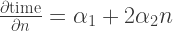
As we see, is a constant effect of scale, while is an effect that varies on the size of n. If is negative, we have a smaller effect as n grows and vice-versa.

It’s also interesting to look at :

where is the expected value. In this model, the effect of changing algorithms is supposed to be constant for any .

Let’s run this on GNU R:


model<-lm(time~n+I(n^2)+f, data=data)
summary(model)

This will give us

Call:
lm(formula = time ~ n + I(n^2) + f, data = data)

Residuals:
     Min       1Q   Median       3Q      Max 
-12.2097  -7.6267  -0.5312   7.7528  12.6358 

Coefficients:
              Estimate Std. Error t value Pr(>|t|)    
(Intercept)  1.190e+01  5.042e+00   2.361   0.0222 *  
n           -9.796e-04  3.860e-03  -0.254   0.8007    
I(n^2)       3.618e-06  6.534e-07   5.537 1.14e-06 ***
f           -2.265e+01  2.273e+00  -9.968 1.79e-13 ***
---
Signif. codes:  0 '***' 0.001 '**' 0.01 '*' 0.05 '.' 0.1 ' ' 1 

Residual standard error: 8.35 on 50 degrees of freedom
Multiple R-Squared: 0.9386,	Adjusted R-squared: 0.9349 
F-statistic: 254.9 on 3 and 50 DF,  p-value: < 2.2e-16 

The estimate column holds the value for the parameters defined on the equation above. The t value column is a measure of how far the parameter is from zero given its uncertainty. If the regression residuals follow a gaussian normal distribution, 1.96 (or -1.96) is a good critical value for considering the variable in question significant; in any case, values above 3 tend to indicate an important relationship.

The effect of is apparently zero, but is significant and positive — which means the algorithm grows more-than-linearly on size. The effect of is very strongly negative, which indicates the second algorithm really tends to be faster.

We can run, just for kicks, the same regression for memory usage. The algebraic analysis remains the same.

Call:
lm(formula = bytes ~ n + I(n^2) + f, data = data)

Residuals:
       Min         1Q     Median         3Q        Max 
-624215565 -421792810   -1493863  425410175  622244685 

Coefficients:
              Estimate Std. Error t value Pr(>|t|)    
(Intercept)  6.368e+08  2.753e+08   2.313  0.02485 *  
n           -2.654e+04  2.107e+05  -0.126  0.90027    
I(n^2)       9.829e+01  3.567e+01   2.755  0.00816 ** 
f           -1.250e+09  1.241e+08 -10.075 1.25e-13 ***
---
Signif. codes:  0 '***' 0.001 '**' 0.01 '*' 0.05 '.' 0.1 ' ' 1 

Residual standard error: 455900000 on 50 degrees of freedom
Multiple R-Squared: 0.8419,	Adjusted R-squared: 0.8324 
F-statistic: 88.77 on 3 and 50 DF,  p-value: < 2.2e-16 

Compare the multiple value between the two regressions. The statistic measures how closely the model fits the data. One way to look at this is to affirm that apparently memory usage is also determined by something else we haven’t mentioned — this evidently being the size of the divisor list.

5. A better model

Let’s revise our equation.

We’ve added an additional “interaction” term. To see what this means, let’s look at expected values again:

In this new model, the effect of changing algorithms is allowed to vary with the size of as well. Let’s estimate this model:

Call:
lm(formula = time ~ n + I(n^2) + f + f:n, data = data)

Residuals:
     Min       1Q   Median       3Q      Max 
-4.56081 -1.30100  0.09815  1.67459  4.00706 

Coefficients:
              Estimate Std. Error t value Pr(>|t|)    
(Intercept) -5.622e+00  1.377e+00  -4.083 0.000164 ***
n            4.451e-03  9.600e-04   4.636 2.66e-05 ***
I(n^2)       3.618e-06  1.592e-07  22.723  < 2e-16 ***
f            1.240e+01  1.362e+00   9.100 4.19e-12 ***
n:f         -1.086e-02  3.856e-04 -28.163  < 2e-16 ***
---
Signif. codes:  0 '***' 0.001 '**' 0.01 '*' 0.05 '.' 0.1 ' ' 1 

Residual standard error: 2.035 on 49 degrees of freedom
Multiple R-Squared: 0.9964,	Adjusted R-squared: 0.9961 
F-statistic:  3418 on 4 and 49 DF,  p-value: < 2.2e-16 

Now all the coefficients are indeed very significant, including the linear term on . This gives us the following formulas for predicting the running time of both algorithms on a given :

An interesting observation: the coefficient for being positive means that the running time of the GCD algorithm starts lower; on the other hand, MOD will quickly outrun it (solve a simple inequality to find ranges of if you’re so inclined).

Conclusions

I might return to this topic if it arises enough interest. For the time being, I tried keeping it short and sweet, even if it meant glossing over all the relevant theoretical details. Discussion is appreciated, etc. etc. Oh, and remember this all was run on an old G4 mac mini, on the interpreter (not compiled/optimized), all while browsing and IMing at the same time. Don’t just benchmark this on JRuby on your dual Opteron and say your language leaves my language biting the dust.

Ok, now I have one more reason not to move out from WordPress.com

The LaTeX people should, by now, have a simple “web” version of LaTeX that can be easily installed by dropping files in your cgi-bin directory. The vast majority of people with hosting services that won’t grant them shell access can’t ever have LaTeX because the current distributions are so desktop-oriented.

bikes.hs

The why parameter passed to the data constructor when you’re using the full syntax as in the jane example is a predicate that decides whether or not color a node yellow. Simple, color-less graphs can be produced with the auxiliary function graph.

Q: How many people with ADD does it take to change a lightbulb?
A: HEY! Let’s ride bikes!


module Bikes where


Graphviz is fun. Graphviz is fair. You may already have one. You may already be there:


data Arr a = a :-> a


Graphviz plots graphs from .DOT files consisting of remarkably simple syntax:


instance (Show a) => Show (Arr a) where show (x:->y) = show x ++ " -> " ++ show y
class (Show a) => (Dot a) where
dot :: [a] -> String
dot = (++"}") . ("digraph untitled {"++) . unlines . map ((++";") . show)
instance (Show a) => Dot (Arr a)


One fun thing we can do with it is plotting graphs of integer-valued functions:


arr f = (\x-> x :-> f x)
rra f = (\x-> f x :-> x)


Let’s see what a simple invertible function looks like:


t2 = dot $ map (arr (*2)) [0..40]


Clearly there’s one and only one way to connect any given two nodes — which is what invertibility means. But let’s look at something fun now; say, the co-totient function. There’s a closed-form equation for this, but why not go full ape declarative?


totient x = x - (length $ [n | n<-[1..x], coprimes n x]) where coprimes a b = (gcd a b) == 1
t3 = dot $ map (arr totient) [1..100]


(Click to see full-size picture)

The first hierarchy line contains the prime numbers; their co-totient is always 1. These numbers are connected to numbers whose co-totient they are; from that graph you can find the co-totient of any number by looking at which number it’s connected to. At first glance it looks pretty tree-like, but it suffices to chase the series of powers of two to see it isn’t.

Now, being that the totient is the quantity of numbers “strange” to a number (in the sense their only common divisor is 1) and the co-totient is precisely a number minus its totient, higher co-totients seem to indicate a more “composite” structure. That’s not clearly represented by graph hierarchy, of course. So we try a different representation of compositeness in integers:


t4 = dot $ filter (\(x:->y) -> y /=1 && x/=y ) $ concat $ map (\y->(map (arr (gcd y)) [2..32])) [2..32]


This will connect all numbers that divide each other by as many arrows as there are ways to divide it:

Click here to see full image

That makes for a smashing bedroom poster.

Finally, as hopelessly amateur mathematicians we are, we just can’t resist poking the Collatz function!


t = dot $ map (rra (\x->if (odd x) then 3*x+1 else x `div` 2)) [1..384]


I’ve plotted Collatz graphs as far as 15000. But let’s keep it to manageable sizes; you can later experiment at home and see trust me that larger graphs keep the structure contained in this graph — there are relatively very few ways to get into the “main Collatz stream” down to 4-2-1 and most numbers are stuck in two-house citadels of their own, with a few managing to form their own substreams that sometimes even manage to join the main Collatz “stream”:

Abandon all hope ye who enter here

Yes, I know, I should be working in PFP and all, but when a boy’s mind is overcome with newfound love, he must clutch at any tiny window of intellectual focus he occasionally comes across by as his brain walks through the shadows of love.


mapM (\x->[x+i | i<-[-5..5]]) [1..5]


No, really, try it. This has to qualify as the “most surprisingly long output” line of code in all of computer programming.