| CARVIEW |
| RAW | REVERSE | |||||||||||
| Subject | 1 | 2 | 3 | 4 | 5 | 1 | 2 | 3 | 4 | 5 | ||
| 25 | 1 | 0 | 38 | 0 | 0 | 0 | 0 | 38 | 0 | 1 | ||
| 200 | 0 | 0 | 38 | 1 | 0 | 0 | 0 | 38 | 1 | 0 | ||
| 230 | 6 | 0 | 33 | 0 | 0 | 4 | 0 | 33 | 0 | 2 | ||
| 353 | 0 | 0 | 35 | 0 | 4 | 2 | 0 | 35 | 0 | 2 | ||
| 422 | 0 | 0 | 0 | 37 | 2 | 1 | 12 | 0 | 25 | 1 | ||
| 445 | 0 | 0 | 28 | 11 | 0 | 0 | 4 | 28 | 7 | 0 | ||
| 448 | 0 | 0 | 0 | 22 | 17 | 6 | 7 | 0 | 15 | 11 | ||
| 460 | 0 | 0 | 9 | 30 | 0 | 0 | 9 | 9 | 21 | 0 | ||
| 465 | 0 | 0 | 38 | 0 | 1 | 0 | 0 | 38 | 0 | 1 | ||
| 469 | 0 | 0 | 19 | 20 | 0 | 0 | 4 | 19 | 16 | 0 | ||
| 473 | 0 | 0 | 1 | 38 | 0 | 0 | 13 | 1 | 25 | 0 | ||
| 520 | 0 | 0 | 36 | 0 | 3 | 0 | 0 | 36 | 0 | 3 | ||
| 655 | 0 | 2 | 0 | 0 | 37 | 12 | 1 | 0 | 1 | 25 | ||
| 662 | 0 | 0 | 0 | 2 | 37 | 11 | 2 | 0 | 0 | 26 | ||
| 779 | 0 | 0 | 33 | 0 | 6 | 0 | 0 | 33 | 0 | 6 | ||
| 828 | 0 | 0 | 9 | 30 | 0 | 0 | 9 | 9 | 21 | 0 | ||
| 856 | 25 | 0 | 0 | 0 | 14 | 20 | 0 | 0 | 0 | 19 | ||
| 914 | 0 | 0 | 0 | 17 | 22 | 7 | 6 | 0 | 11 | 15 | ||
| 929 | 0 | 0 | 21 | 18 | 0 | 0 | 7 | 21 | 11 | 0 | ||
| 938 | 0 | 0 | 36 | 0 | 3 | 0 | 0 | 36 | 0 | 3 | ||
| 939 | 0 | 0 | 36 | 3 | 0 | 0 | 0 | 36 | 3 | 0 | ||
| 997 | 0 | 14 | 0 | 25 | 0 | 0 | 19 | 0 | 20 | 0 | ||
]]>
No, I don’t have any references because I did not look for any. However, I can give you some visual examples of this unequal variability property.
For a while now, I have been studying daily station series and it seems quite clear that winter temperatures are more variable than summer ones and that this effect is very strongly accentuated as one moves toward the poles. Recently BEST published their newly minted temperature series and at their web page, they produced a gridded equal-area cell construction of 5498 monthly land temperature series.
I took a time-truncated subset of all of these series starting in February, 1956 (the date was chosen because it was the earliest date from which all of the cells had values for each month) and continuing to the most recent values. For each series, the standard deviation of the temperature was calculated separately for each month.
The first pair of plots gives a plot of the SD by latitude for the months of February and August. The red lines are references for the tropics.

The second pair is a plot versus longitude with point from the northern and southern hemisphere indicated by color.

Admittedly, I have not detrended the anomalies first, but the climate variation for a cell should not be large enough to create such large differences in the SDs between months.
Unequal variability would create a fairly substantial stumbling block for finding changepoints in series.
]]>Papers were published by Steve McIntyre and Ross McKitrick showing that the centering methods used in the Mann papers produced statistically biased results. Questions were raised about the proxies used and it became evident that one could produce similar “temperature” series by utilizing certain types of artificially generated random series rather than physical proxies which purportedly were related to the temperatures. This eventually led to a congressional hearing to establish whether the M & M criticism was valid. Prof. Edward Wegman was commissioned to produce a report examining the various claims.
For further discussion , it is important to understand the makeup of the contents of this report:
Executive summary (5 pages)
Introduction (3 pages)
Background on Paleoclimate Temperature Reconstruction (13 pages)
– Includes Paleo Info, PCs, Social networks
Literature Review of Global Climate Change Research (5 pages)
Reconstructions And Exploration Of Principal Component Methodologies (10 pages)
Social Network Analysis Of Authorships In Temperature Reconstructions (10 pages)
Findings (3 pages)
Conclusions and Recommendations (2 pages)
Bibliography (7 pages)
Appendix (33 pages)
– Includes PCA math, Summaries of papers and Sundry
The three topics which have been most discussed on the web include the background explanatory material on proxies (~6 pages), the analysis of the Mann applications of PCA (~16 pages) and the social network analysis (~15 pages which include 9 figures, each of which occupies a major portion of a page).
It should also be understood that these three topics are stand-alone. The material discussed within a topic along with any results obtained is independent of that in each of the others. Therefore, criticism of some aspect of a particular topic will have no bearing on the accuracy or correctness of any portion of the other topics.
The material on social networks was then used in preparing a publication using social networking procedures to relationships among authors in the paleo-climate community. The resulting paper was published in the Journal, Computational Statistics and Data Analysis, about a year later under the authorship of Yasmin H. Said, Edward J.Wegman, Walid K. Sharabati, and John T. Rigsby.
The original report has been a thorn in the side of advocates of Global Warming since it was presented. Many attempts have been made to discredit the report including accusations of plagiarism of parts of a work by R. S. Bradley who made the rather extraordinary demand that the entire report be withdrawn even though, as I point out above, any such use of the material from his work had no impact on other portions of the report.
The concerted effort by the ankle-biters to discredit Prof. Wegman continued until it seems to have resulted in the withdrawal of the social networking paper due to charges that some material in the paper was not properly referenced. The quality of the paper was further discussed in USA Today in an email interview with a “well-established expert in network analysis”, Kathleen Carley of Carnegie Mellon. It is this latter news article that I wish to discuss.
Q: Would you have recommended publication of this paper if you were asked to review it for regular publication — not as an opinion piece — in a standard peer-reviewed network analysis journal?
A: No – I would have given it a major revision needed.
Over the past thirty or so years, there has been a move in the statistical community to present a greater number of papers illustrating applications of newer statistical techniques. These are not papers intended to “move the science forward” as much as to inform other statisticians about the use of the techniques and to often highlight an innovative application of the methodology. As such, they would certainly not be the type of paper submitted to a journal which specialized in the subject matter. This sort of paper may sometimes written by students with their supervisor’s cooperation.
Note the letter Prof. Wegman sent to the editor of the journal:
Yasmin Said and I along with student colleagues are submitting a manuscript entitled ―Social Network Analysis of Author-Coauthor Relationships.This was motivated in part by our experience with Congressional Testimony last summer. We introduce the idea of allegiance as a way of clustering these networks. We apply these methods to the coauthor social networks of some prominent scholars and distinguish several fundamentally different modes of co-authorship relations. We also speculate on how these might affect peer review.
The indication is clear that the paper is intended to present a simple application of the methodology to the wider statistical audience.
Q: (How would you assess the data in this study?)
Data[sic]: Compared to many journal articles in the network area the description of the data is quite poor. That is the way the data was collected, the total number of papers, the time span, the method used for selecting articles and so on is not well described.
I agree that the data is not described in depth in this paper. However, a better description of the data was given in the earlier report in which it was initially used. That report was referenced in the submitted paper, but it is quite possible that it was not read by Prof. Carley.
It should be noted that the authors had decided not to mention any names of the subjects whose author network was analyzed. This would reduce both the type and the amount of information that could be included without violating that anonymity.
Q: (So is what is said in the study wrong?)
A: Is what is said wrong? As an opinion piece – not really.
Is what is said new results? Not really. Perhaps the main “novelty claim” are the definitions of the 4 co-authorship styles. But they haven’t shown what fraction of the data these four account for.
As I mention above, this is an expository presentation of the use of the methodology, NOT an “opinion piece” as characterized by Prof. Carley. No “new results” as such are needed. Furthermore, she does not indicate that the results in the presentation could be incorrect in any way.
There was one other paragraph in the article which caught my attention:
Carley is a well-established expert in network analysis. She even taught the one-week course that one of Wegman’s students took before 2006, making the student the “most knowledgeable” person about such analyses on Wegman’s team, according to a note that Wegman sent to CSDA in March.
Social network methodology is not rocket science. The average statistician could become reasonably proficient in applying the methodology in a relatively short period of time. Understanding the methodology sufficiently to “advance the science” would indeed require considerably more study and time to develop the skills needed. It is unfortunate that the journalist exposed his uninformed biases with a negative comment such as this.
There have been questions about the short review period before the paper was accepted. Dr. Azen indicated in the USA Today article that he personally reviewed and accepted the paper, not a surprise if you take into account my earlier comments about the expository nature of the paper. However, It is unfortunate that he did not demand a more comprehensive bibliography since it is indeed much too sparse. If he had done so, we would likely not even be discussing this subject.
Nonetheless, nobody has demonstrated that the science in the paper has been faulty and, regardless of its demise, the fact stands that the original report and its conclusions regarding the flawed hockey stick cannot be impacted by this is any way.
]]>Second, that in doing the analysis, we retain too few (just 3) EOF patterns. These are decompositions of the satellite field into its linearly independent spatial patterns. In general, the problem with retaining too many EOFs in this sort of calculation is that one’s ability to reconstruct high order spatial patterns is limited with a sparse data set, and in general it does not makes sense to retain more than the first few EOFs. O’Donnell et al. show, however, that we could safely have retained at least 5 (and perhaps more) EOFs, and that this is likely to give a more complete picture.
Some background may be required for the non-statistically oriented reader. A singular value decomposition allows one to take a set of numerical data sequences (usually arranged into a matrix array) and to decompose it into a new set of sequences (called Principal Components or Empirical Orthogonal Functions), a set of weights indicating the amount of variability of the original set accounted for by each of the PCs (called eigenvalues or singular values) and a set of coefficients which relate each PC to each of the original sequences. To reconstruct the original sequences, one can take each PC, multiply it by its eigenvalue and then use the coefficients to reproduce the original data.
This decomposition has certain properties which can be very useful in understanding and analyzing the original data. In particular, when there are strong relationships between the data sequences, several of the eigenvalues may be much larger than the rest. Using only the PCs which belong to those eigenvalues can create a very good replica of the data, but with fewer “moving parts”.
In the Steig paper, the authors divided the Antarctic into 5509 grid cells. They took a huge amount of satellite data and from it formed a monthly temperature sequence ( from January 1982 to December 2006 – 300 months) for each of the grid cells. The problem was to estimate the behavior of various regions of Antarctica during the longer period from January 1957 to the end of 2006 (a total of 600 months). Since the data before the satellite era was sparse both geographically and temporally, it was decided to try to “extend” the satellite data to the earlier period by first relating it to the ground temperatures that were available and then using that relationship to guess what the satellite temperatures might have been prior to 1982.
This is a good idea, but, as always, the devil is in the details. Using the totality of the available satellite sequences was unwieldy, both from a mathematical and statistical standpoint. This is where the decision to use a PC approach came in handy. The satellite temperature sequences have a great deal of relationship within their structure. For example, one would expect that geographically adjacent grid cells would have very similar behavior so it was apparent that this approach could reasonably produce something useful.
How many PCs should one use? This is the specific disagreement mentioned in the above quote from the RC post. Too many PCs mean a larger number of values to be estimated from the earlier station data (300 for each PC wherein the “overfitting” claim arises). On the other hand, too few PCs mean that the reconstruction will be unable to properly separate the spatial and temporal temperature patterns. The temperatures from the peninsula can be “smeared” to West Antarctica, there could be no ability to make separate examinations of the temperatures during the various seasons or any combination of these items.
One could argue that the graph from Odonnell et al. displayed in the RC post illustrates this difference:

Too few PCs will produce a monotone colored plot: With a single PC, every grid cell will have exactly the same characteristics since only a single multiplier and a single PC are available to reconstruct it. With two PCs, only two coefficients are available to differentiate the entire cell sequence from all of the others, etc. As more PCs are added, more variation in the coloring becomes possible. Whether this represents a greater reality or not becomes an issue.
What method should be used to “establish the relationship” between the satellites and the ground and to extend the sequences to the pre-1982 era? There are several of these that are available. They have different properties and it is important to understand what the drawbacks of each can be. The two mentioned in the RC post are TTLS (truncated total least squares – advocated by Mann and Steig) and ‘iridge’ (individual ridge regression – part of the methodology used by OD 2010). Discussion of these is a complicated matter which is beyond the discussion here.
The point of this post is to look at the specific 3 PCs which were used by the Steig paper. One can download the Antarctic reconstruction from the papers web site (warning –it is a VERY large text file) and using the R svd function decompose it using a singular value decomposition. Since the means of the sequences are not all zero, the “PCs” are not orthogonal, but it does not impact the point being made here. A plot of the 3 PCs used by Steig et al (oriented so that all trends are positive) produce the following:

The third PC looks somewhat different from the other two. The (extended) portion prior to 1982 is pretty close to being identically zero. Any reconstruction of the satellite data using these PCS becomes essentially a two PC reconstruction prior to 1982 and three PCs afterward. The end effect of the third PC on the overall results is to put a bend in the trends at that point (upward if the coefficient is positive and down if negative).
However, can this reconstruction differentiate well between the Antarctic regions in the early temperature record? I sincerely doubt it unless someone believes that the record is sufficiently homogeneous both spatially and temporally to justify that possibility. Perhaps, the authors of Steig et al. could explain this in more detail – I presume that they would have seen the same graph when they were writing the paper.
Why did this occur? My best guess is that it might be a result of using the total least squares function in the procedure.
I will give three more plots. Each of these is a plot of the relative size of the grid cell coefficient for each of the PCs when combining them to create the three PC satellite series. NOTE: These are NOT the values of the trends.

PC1 produces a general increasing trend throughout the continent. This trend is somewhat more pronounced in the central area.

PC2 is the main driver for the peninsula – West Antarctica relationship.

The main effects of this are felt after 1982 – it adds to the cooling lower right and the warming upper left.
]]>A brief explanation of the difference between ordinary least squares (OLS) and EIV is in order. Some further information can be found on the Wiki Error-in-Variables and Total least squares pages. We will first look at the case where there is a single predictor.
Univariate Case
The OLS model for predicting a response Y from a predictor X through a linear relationship looks like:

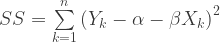
α and β are the intercept and the slope of the relationship, e is the “random error” in the response variable due to sampling and/or other considerations and n is the sample size. The model is fitted by choosing the linear coefficients which minimize the sum of the squared errors (which is also consistent with maximum likelihood estimation for a Normally distributed response:
The problem is easily solved by using matrix algebra and estimation of uncertainties in the coefficients is relatively trivial.
EIV regression attempts to solve the problem when there may also be “errors”, f, in the predictors themselves:

The f-errors are usually assumed to be independent of the e-errors and the estimation of all the parameters is done by minimizing a somewhat different looking expression:

under the condition

X* and Y* (often called scores) are the unknown actual values of X and Y. The minimization problem can be recognized as calculating the minimum total of the perpendicular squared distances from the data points to a line which contains the estimated scores. Mathematically, the problem of calculating the estimated coefficients of the line can be solved by using a principal components calculation on the data. It should be noted that the data (predictors and responses should each be centered at zero beforehand.
The following graphs illustrate the difference in the two approaches:

What could be better, you ask. Well, all is not what it may seem at first glance.
First, you might have noticed that the orange lines connecting the data to the scores in the EIV plot are all parallel. The adept reader can see from considerations of similar triangles that the ratio of the estimated errors, e and f (the green lines plotted for one of the sample points), is a constant equal to minus one times the slope coefficient (or one over that coefficient dependent on which is the numerator term). The claim that somehow this regression properly takes into account the error uncertainty of the predictors seems spurious at best.
The second and considerably more important problematic feature is that, as the total-least squares page of Wiki linked above states: “total least squares does not have the property of units-invariance (it is not scale invariant).” Simply put, if you rescale a variable (or express it in different units), you will NOT get the same result as for the unscaled case. Thus, if we are doing a paleo reconstruction and we decide to calibrate to temperature anomalies as F’s rather than C’s, we will end up with a different reconstruction. How much different will depend on the details of the data. However, the point is that we can get two different answers simple by using different units in our analysis. Since all sorts of rescaling can be done on the proxies, the end result is subject to the choices made.
To illustrate this point, we use the data from the example above. The Y variable is multiplied by a scale factor ranging from .1 to 20. The new slope is calculated and divided by the old EIV slope which has also been scaled by the same factor.

If the procedure was invariant under scaling (as OLS is), then the result should be equal to unity in all cases. Instead, one can see that for scale factors close to zero, the EIV behaves basically like ordinary OLS regression . As the scale factor increases, the result (after unscaling) looks like 1/the OLS slope with the X and Y variables switched.
However, that is not the end of the story. What happens if both X and Y are each scaled to have standard deviation 1? This surprised me somewhat. The slope can only take either +1 or -1 (Except for some cases where the data form an exactly symmetric pattern for which ALL slopes produce exactly the same SS).
In effect, this would imply that, after unscaling , the EIV calculated slope = sd(Y) / sd(X). To a statistician, this would be very disconcerting since this slope is not determined in any way shape or form by any existing relationship between X and Y – this is the answer when the data points are in an exactly straight line or when they are uncorrelated. It is not affected by sample size so clearly large sample convergence results would not be applicable. On the other hand, the OLS slope = Corr(X,Y) * sd(Y) / sd(X) for the same case so that this criticism would not apply to that result.
Multilinear Case
So far we have only dealt with the univariate case. Perhaps if there are more predictors, this would alleviate the problems we have seen here. All sorts of comparisons are possible, but to shorten the post, we will only look at the effect of rescaling the all of the variables to unit variance.
Using R, we generate a sample of 5 predictors and a single response variable with 20000 values each. The variables are generated “independently” (subject to the limits of a random number generator). We calculate the slope coefficients for both the straight OLS regression and also for EIV/TLS:
| Variable | OLS Reg | EIV-TLS |
| X1 | 0.005969581 | 1.9253757 |
| X2 | 0.010657532 | 1.8661962 |
| X3 | -0.005656248 | 3.7607298 |
| X4 | -0.003537972 | 0.6509362 |
| X5 | 0.003616522 | 4.4236177 |
All of the theoretical coefficients are supposed to be zero and with 20000 observations, the difference should not be large. In fact 95% confidence intervals for the OLS coefficients all contain the value 0. However, the EIV result is completely out to lunch. The response Y must be scaled down by about 20%, to have all of the EIV coefficients become small enough to be inside the 95% CIs calculated by the OLS procedure.
EIV on Simulated Proxy Data
We give one more example of what the effect of applying EIV in the paleo environment can be.
As I mentioned earlier, I have been looking at the response by Gavin and crew to the M-W paper. In their response, the authors use artificial proxy data to compare their EIV construct to other methods. Two different climate models are used to generate a “temperature series” and proxies (which have auto-regressive errors) are provided. I took the CSM model (time frame used 850 to 1980) with 59 proxy sequences as the data. An EIV fit with these 59 predictors was carried out using the calibration period 1856 to 1980. A simple reconstruction was calculated from these coefficients for the entire time range.
This reconstruction was done for each of the three cases: (i) Temperature anomalies in C, (ii) Temperature anomalies in F, and (iii) Temperature anomalies scaled to unit variance during the calibration period. The following plots represent the difference in the resulting reconstructions: (i) – (ii) and (i) – (iii):

The differences here are non-trivial. I realize that is not a reproduction of the total method used by the Mann team. However, the EIV methodology is central to the current spate of their reconstructions so some effect must be there. How strong is it? I don’t know – maybe they can calculate the Fahrenheit version for us so we can all see it. Surely, you would think that they would be aware of all the features of a statistical method before deciding to use it. Maybe I missed their discussion of it.
A script for running the above analysis is available here (the file is labeled .doc, but it is a simple text file). Save it and load into R directly: Reivpost
]]>
There has been a flurry of activity during the last several months in the area of constructing global temperature series. Although a variety of methods were used there seemed to be a fair amount of similarity in the results.
Some people have touted this as a “validation” of the work performed by the “professional” climate agencies which have been creating the data sets and working their sometimes obscure manipulation of the recorded temperatures obtained from the various national meteorological organizations that collected the data. I for one do not find the general agreement too surprising since most of us have basically used the same initial data sets for our calculations. I decided to take a closer look at the GHCN data since many of the reconstructions seem to use it.
At this point, I will look at some of the data which can be found in the GHCN v2.mean.z file. This represents monthly mean temperatures calculated for a collection of temperature stations around the globe. People tend to refer to these as “raw” data, but statistically this is not really the case. Each monthly record represents a calculated value of a larger set of data. The means can be calculated in different ways. Since there can be missing daily values due to equipment malfunctions and other reasons, decisions have been made and implemented in how to do the calculation in such cases. It is very possible that further “adjustments” may have also been made before the data reaches GHCN.
A description of the format of all the temperature datasets is given in the readme file at the same site. In particular, station series id formats are as follows:
Each line of the data file has:
station number which has three parts:
country code (3 digits)
nearest WMO station number (5 digits)
modifier (3 digits) (this is usually 000 if it is that WMO station)Duplicate number:
one digit (0-9). The duplicate order is based on length of data.
Maximum and minimum temperature files have duplicate numbers but only one time series (because there is only one way to calculate the mean monthly maximum temperature). The duplicate numbers in max/min refer back to the mean temperature duplicate time series created by (Max+Min)/2.
In this analysis, I will be referencing the station with a single id which is constructed from the station number by connecting it to the modifier with a period. The temperature data in the R program will consist of a list of (possibly multivariate) time series with each element of the list containing all of the “duplicates” for a particular station.
Some “quality control” has also been done by GHCN. The earlier “readme” also explains the file v2.mean.failed.qc.Z:
Data that have failed Quality Control:
We’ve run a Quality Control system on GHCN data and removed data points that we determined are probably erroneous. However, there are some cases where additional knowledge provides adequate justification for classifying some of these data as valid. For example, if an isolated station in 1880 was extremely cold in the month of March, we may have to classify it as suspect. However, a researcher with an 1880 newspaper article describing the first ever March snowfall in that area may use that special information to reclassify the extremely cold data point as good. Therefore, we are providing a file of the data points that our QC flagged as probably bad. We do not recommend that they be used without special scrutiny. And we ask that if you have corroborating evidence that any of the “bad” data points should be reclassified as good, please send us that information so we can make the appropriate changes in the GHCN data files. The data points that failed QC are in the files v2.m*.failed.qc. Each line in these files contains station number, duplicate number, year, month, and the value (again the value needs to be divided by 10 to get degrees C). A detailed description of GHCN’s Quality Control can be found through https://www.ncdc.noaa.gov/ghcn/ghcn.html.
I didn’t really find the “detailed description”, but a check of the file indicated that almost all of the entries in the file represented temperature values that had been removed from the data set (replaced by NAs). I could only find seven monthly temperatures where the original value was replaced by a new one. Without the necessary supplementary metadata, there is no sense at looking at that file any further.
The names of the stations and other geographic data for them can be found in the v2.temperature.inv file. There are 7280 stations listed with 4495 unique WMO numbers. Each station can have one or more (up to a maximum of 10) “duplicates” so there are a total of 13486 temperature series in the data set. The duplicate counts look like:
| Dups: | 1 | 2 | 3 | 4 | 5 | 6 | 7 | 8 | 9 | 10 |
| Freq: | 4574 | 1109 | 601 | 502 | 269 | 111 | 56 | 44 | 12 | 2 |
Before the data can be used to construct the global record, it is necessary to somehow combine the information from the various duplicate versions into a single series. One reasonably expects that the duplicates should be pretty much identical (with the occasional error) since they are supposedly different transcriptions of the same temperature series. The difficulty is that there are almost 13500 series which have to be looked at – not a simple matter.
The 4574 stations which were represented by a single series can be ignored for the moment – there is little that can be done to evaluate – so, for simplicity, I decided to only look at the “twins”, i.e. those 1109 stations which have exactly two records. These were identified and the range for the simple difference between the two series was calculated. No heavy duty stats were necessary to take a look at the amount of agreement there was between them.
I expected most of the stations to look like this:

However, there were others that looked like this one:

How many? Well that was the surprise! I graphed those which were not identical over their overlap periods and put the graphs into pdfs.
No overlap: 232 stations (no plots)
Zero difference: 152 stations (no plots)
Range between 0 and 1- : 233 stations (4.9 MB pdf)
Range between 1 and 3- : 321 stations (6.9 MB pdf)
Range between 3 and 12.9 : 171 stations (4.1 MB pdf).
The latter two files are the more interesting ones. “Duplicate” has taken on a whole new meaning for me.
If there are any errors in my results, R scripts or explanations of the phenomena in the plots, I would like to hear about them.
I have uploaded the R script as an ordinary text file called twin analysis.doc.
]]>Arctic sea ice extent averaged 13.10 million square kilometers (5.06 million square miles) for the month of May, 500,000 square kilometers (193,000 square miles) below the 1979 to 2000 average. The rate of ice extent decline for the month was -68,000 kilometers (-26,000 square miles) per day, almost 50% more than the average rate of -46,000 kilometers (18,000 square miles) per day. This rate of loss is the highest for the month of May during the satellite record.
However, later on the same page, they also state under Conditions in Context:
As we noted in our May post, several regions of the Arctic experienced a late-season spurt in ice growth. As a result, ice extent reached its seasonal maximum much later than average, and in turn the melt season began almost a month later than average. As ice began to decline in April, the rate was close to the average for that time of year.
In sharp contrast, ice extent declined rapidly during the month of May. Much of the ice loss occurred in the Bering Sea and the Sea of Okhotsk, indicating that the ice in these areas was thin and susceptible to melt. Many polynyas, areas of open water in the ice pack, opened up in the regions north of Alaska, in the Canadian Arctic Islands, and in the Kara and Barents and Laptev seas.
This latter observation that the seasonal maximum was reached later in the season and the melt season started later is important. Regardless of specific annual weather conditions, May and June are melt season months in the Arctic. Furthermore, if there is more ice available, then it stands to reason that more melting will take place. What might a better way to look at the data than simply plotting the total extent?
From the JAXA site:

Why not graph the rate of change, as well? In particular, because a wider extent will naturally imply a higher areal melt under the same melting conditions, it makes sense to look at the daily percentage change.
To do this, I downloaded the JAXA daily ice data into R (from 2002 to the present). For convenience purposes, December 31 was deleted from both 2004 and 2008 to reduce the number of days to 365. The percentage change was calculated for each day for which the corresponding data was available. No infilling was done for missing data. The data was plotted:
(Click graph for larger version)

Here, all of the years prior to 2010 are plotted in gray and the current year in red. The plot gives graphic insight into the patterns of thawing and freezing: the thaw season goes from roughly mid-March to mid-September. The very high variability in October is likely due to a reasonably similar annual speed of recovery which is expressed as a percentage of quite varied minima starting points in September.
How does 2010 compare in May and June? For May, it is somewhat toward the lower part the combined record, but I would not classify it as extreme in any way. June was definitely below the other recent years during three periods of several days each. What will July and August look like? I guess we will have to wait and see…
The R script follows:
#get latest JAXA extent data
iceurl = url("https://www.ijis.iarc.uaf.edu/seaice/extent/plot.csv")
latest = read.csv(iceurl,header=F,na.strings="-9999")
colnames(latest) = c("month","day","year","ext")
#remove Dec 31, 2004 and 2008 (extra leap year day) for convenience
#fill in with missing values for early part of 2002 (for convenience)
arc.ext = latest$ext
which((latest$month==12)&(latest$day==31)) # 214 579 945 1310 1675 2040 2406 2771 3136
arc.ext = arc.ext[-c(945,2406)]
arc.ext = c(rep(NA,365-214),arc.ext)
#length(arc.ext)/365 # 9
#calculate changes as % of current value
#form matrix with 9 columns (one for each year)
pct.change = matrix(100*c(diff(arc.ext),NA)/arc.ext,ncol=9)
#plot data
#years 2002 to 2009 as gray background
#year 2010 in red
#add month boundaries
modays = c(31,28,31,30,31,30,31,31,30,31,30,31)
matplot(pct.change[,1:9],type="l",main ="Arctic ice Extent Change Relative to Area",xlab="Day",
ylab="Daily % Change", col=c(rep("grey",8),"red"),lty=1)
abline(h=0)
abline(v=c(0,cumsum(modays)), col="green")
text(x =14+c(0,cumsum(modays)[-12]),y =c(rep(3,9),rep(-1,3)), labels=month.abb,col="blue")
I had been testing some methods for estimating the temperature at particular locations in a geographic grid cell from the temperature data set released by the Met Office. The grid cell was chosen on the basis that was a reasonable collection of stations available for use in the procedure: 40 – 45 N by 100 – 105 W in the north central region of the United States. I chose a station with a longer fairly complete record and my intent was to look at distance based weighting for estimating the temperature at that station site using the neighboring stations. Then I could compare the actual measured temperature to the estimated temperature to evaluate how well I had done. But my results seemed poorer than I had expected. At that point, I thought that perhaps I should look more closely at the station record.
The station I had chosen was Rapid City, South Dakota – ID number 726620 with a current population close to 60000 people according to Wikipedia . For comparison purposes, I collected the same station’s records from a variety of other sources: GISS “raw” (same as “combined”) and homogenized directly from the Gistemp web pages, GHCN “raw” and adjusted from the v2 data set and what was listed as the same two GHCN records from the Climate Explorer web site. The subsequent analysis proved quite interesting.
To start with, the data from the Climate Explorer web site proved to be identical to the GHCN data that it purported to be. A plot of the remaining five data sets looks like this:

At a glance, the records look quite similar with what appear to be some minor variations particularly in the later portions of the series. Next, I compared the effects of the adjustments made in the case of GISS and GHCN.

This proved rather interesting. Whereas the GISS homogenization was a simple increase of about 0.4 degrees in several stages, nothing we haven’t seen before. However, the GHCN adjustment is quite complicated so a further plot of the adjustments by month seemed to be a good idea.
Monthly GHCN Adjustments:

Now this I find difficult to understand. The pattern of the adjustments differs substantially for the various months with a strongly induced increasing trend in the summer and fall. Since it is unlikely that the station is moved each spring to another location (the weatherman’s summer residence?  ) and then back into town in the fall, I cannot find a reasonable explanation for either the type or the amounts of the adjustment. However, it was downhill from here.
A comparison of GISS to GHCN:

None of the GISS series is even close to either of those from GHCN! Yet they all purport to be the temperatures measured at a single site. However, we have forgotten the Met series which initiated the entire exercise. Met Office’s version compared to the other four:

Well, not only different, but in a strange way. Starting in the early 1980’s, met decides to go off on its own. Where the other four series have missing values (consistent with each other), Met always has a measurement available. As well, the difference between Met and the others at times becomes relatively large.
As a final step, I calculated the trends from 1970 onwards for each of the five. On a decadal basis:
Met 0.021 C / decade
GISS 0.167 C / decade
Homogenized GISS 0.253 C / decade
GHCN -0.185 C / decade
Adjusted GHCN 0.302 C / decade
Why are they all so different? I haven’t got a clue! I triple-checked the data sources, but couldn’t find any errors in my versions of the data. Maybe someone out there can provide some enlightenment.
I hope the rest of the records are not like this…
The data I used are on the website and can be downloaded through the script below.
#get data

rapiddat = url("https://statpad.wordpress.com/wp-content/uploads/2010/03/rapidcity.doc")
rapidcityx = dget(rapiddat)

rapidcity = rapidcityx[,1:5]

plot(rapidcity) #rapid1

par(mfrow=c(2,1))

#giss is raw and/or combined sources)
#rapid2
plot(rapidcity[,"homgiss"]-rapidcity[,"giss"], main = "GISS ... Homogenized  - Raw",xlab="Year",ylab = "Degrees C" )

plot(rapidcity[,"adjghcn"]-rapidcity[,"ghcn"],main = "GHCN ... Adjusted  - Raw",xlab="Year",ylab = "Degrees C")

#monthly pattern of diffs for ghcn rapid3
par(mfrow=c(4,3))
for (i in 1:12) {
 plot(window(rapidcity[,"adjghcn"]-rapidcity[,"ghcn"], start=c(1888,i),deltat=1),ylim=c(-2,1),main = month.name[i],ylab ="Degrees C",xlab="Year")
 abline(h=0,col="red")}

par(mfrow=c(2,2))

plot(rapidcity[,"giss"]-rapidcity[,"ghcn"], main = "GISS - GHCN",xlab="Year",ylab = "Degrees C" )
plot(rapidcity[,"homgiss"]-rapidcity[,"ghcn"],main = "Homogenized GISS - GHCN",xlab="Year",ylab = "Degrees C")
plot(rapidcity[,"giss"]-rapidcity[,"adjghcn"], main = "GISS - Adjusted GHCN",xlab="Year",ylab = "Degrees C" )
plot(rapidcity[,"homgiss"]-rapidcity[,"adjghcn"],main = "Homogenized GISS -  Adjusted GHCN",xlab="Year",ylab = "Degrees C")

par(mfrow=c(2,2))
plot(rapidcity[,"met"]-rapidcity[,"ghcn"], main = "Met - GHCN",xlab="Year",ylab = "Degrees C" )
 abline(h = 0,col="red")
plot(rapidcity[,"met"]-rapidcity[,"adjghcn"],main = "Met - Adjusted GHCN",xlab="Year",ylab = "Degrees C")
 abline(h = 0,col="red")
plot(rapidcity[,"met"]-rapidcity[,"giss"], main = "Met - GISS",xlab="Year",ylab = "Degrees C" )
 abline(h = 0,col="red")
plot(rapidcity[,"met"]-rapidcity[,"homgiss"],main = "Met - Homogenized GISS",xlab="Year",ylab = "Degrees C")
 abline(h = 0,col="red")

#trends
rapid70 = window(rapidcity,start=c(1970,1))
trend = rep(NA,5)
mons = factor(cycle(rapid70))
tim = time(rapid70)
for (i in 1:5) trend[i] = lm(rapid70[,i]~0+mons+tim)$coe[13]
names(trend)=colnames(rapid70)
trend

#         met         giss      homgiss         ghcn      adjghcn
# 0.002050500  0.016706298  0.025326090 -0.018540570  0.030191120
]]>Think about that. We’re re-aligning the anomaly series with each other to remove the steps. If we use raw data (assuming up-sloping data), the steps in this case were positive with respect to trend, sometimes the steps can be negative. If we use anomaly alone (assuming up-sloping data), the steps from added and removed series are always toward a reduction in actual trend. It’s an odd concept, but the key is that they are NOT TRUE trend as the true trend, in this simple case, is of course 0.12C/Decade.
The actual situation is deeper than Jeff thinks. The usual method used by climate scientists for doing monthly anomaly regression is wrong! Before you say, “Whoa! How can a consensus be wrong?”, let me first give an example which I will follow up with the math to show you what the problem is.
We first produce a series of ten years of ten years worth of noiseless temperature data. To make it look realistic (not really important) we will take a sinusoidal annual curve and superimpose an exact linear trend (of .2 degrees per year) on the data:

We now calculate the anomalies and fit a linear regression line to the anomalies. The following is a plot of anomalies with a regression line:

The resulting trend of .198 does not match the actual trend in the data despite the fact that there is no noise present in the series. Although the difference in this case is not large (a poor oft-repeated justification), this is an uncorrectable bias error. What is not as obvious is that this will have an impact on the autocorrelation in the situation as evidenced by the ACF of the residuals – an effect due to the methodology and not inherent to the actual “error” sequence:

But it gets worse. If we change our starting month (but still use ten full years of data), we get different slopes for each month:
| Month | Intercept | Trend |
| 1 | -1.27983 | 0.198014 |
| 2 | -1.28521 | 0.198931 |
| 3 | -1.28971 | 0.199681 |
| 4 | -1.29331 | 0.200264 |
| 5 | -1.29595 | 0.200681 |
| 6 | -1.2976 | 0.200931 |
| 7 | -1.29822 | 0.201014 |
| 8 | -1.29775 | 0.200931 |
| 9 | -1.29618 | 0.200681 |
| 10 | -1.29344 | 0.200264 |
| 11 | -1.2895 | 0.199681 |
| 12 | -1.28431 | 0.198931 |
The average is equal to .2 so all is not lost. However, all of the errors are a result of how we chose to do our analysis and were not really present in the original data.
So what’s causing the problem?
Here comes the math
What most climate scientists still do not seem to understand is the need to spell out the parameters and how they relate to each other. Unless such a “statistical model” exists, we do not have a good grasp of what is happening when we carry out an analysis and a reduced ability to recognize when something is not quite right. The implicit model in this situation is

where
X(t) = temperature at time t
t = y + m, where y = year and m = month (with values 0/12 , 1/12, …,11/12)
µm = mean of month m
β = annual trend
ε(t) = “error” (which in this case are all zeroes).
Now, what happens when we calculate anomalies? If A(t) is the anomaly at time t,

where the “bar” represents averaging over that variable.
Here,

and if we substitute this in the original equation we get

The important thing to realize here is the the month no longer appears with the trend – only the year (and NOT time) should be used to get the correct trend. By using time, we actually are fitting the line

for which the intercept should be different for each month. Since the usual anomaly regression fits a single intercept, the resulting trend is incorrectly estimated.
How can this be fixed?
Several fixes are possible. The simplest is to use year rather than time as the independent variable in the regression. This may seem counterintuitive, but it takes the anomalies and lines then up vertically above each other solving the problem that Jeff noticed. However, this solution can still be problematical if the number of available anomalies differs from year to year.
A better solution is to do the anomalizing and the trend fit at the same time. This corresponds to a single factor Analysis of Covariance where month is treated as a categorical factor with twelve levels and time (or year!) is treated as a numeric covariate. This can be implemented in R using the function lm.
The script used in the post follows:
#we construct 11 years of data for later use
seasonal = 5 + 10*sin(pi*(0:131)/6)
#add trend of .2 degrees per year
trend = (0:131)/60

temps = ts((seasonal+trend)[1:120],start=c(1,1),freq=12)
time.temp= time(temps)

plot(seasonal,type="l")

plot(temps, main="Plot of Monthly Temperature Time Series", ylab="Degrees C", xlab="Time") #anomregfig1.jpg

#function to calculate anomaly
anomaly.calc=function(tsdat,styr=1951,enyr=1980){
 tsmeans = rowMeans(matrix(window(tsdat,start=c(styr,1),end=c(enyr,12)),nrow=12))
 tsdat-rep(tsmeans,len=length(tsdat))}

anom = anomaly.calc(temps,1,10)

#anomaly regression
reg1 = lm(anom~time.temp) #  intercept =  -1.180, slope = 0.198

plot(anom, main = "Anomalies",ylab = "Degree C",xlab = "Time") #anomregfig2.jpg
abline(reg = reg1,col="red")

#calculate autocorrelation of residuals
acf(residuals(reg1))  #anomregfig3.jpg

#set up revolving regressions
tempsx = ts(seasonal+trend,start=c(1,1),freq=12)
timex.temp= time(tempsx)
anomx.all = anomaly.calc(tempsx,1,11)

#function to cycle regression starting points and give coefficients
cycle.reg = function(dats) {
 coes = matrix(NA,12,2)
 coes[1,] = coef(lm(window(dats,start=c(1,1),end=c(10,12))~time(window(dats,start=c(1,1),end=c(10,12)))))
 for (i in 1:12) coes[i,] = coef(lm(window(dats,start=c(1,i),end=c(11,i-1))~time(window(dats,start=c(1,i),end=c(11,i-1)))))
coes}

(all.coef = cycle.reg(anomx.all))

#           [,1]      [,2]
# [1,] -1.279832 0.1980138
# [2,] -1.285205 0.1989305
# [3,] -1.289710 0.1996805
# [4,] -1.293305 0.2002639
# [5,] -1.295949 0.2006806
# [6,] -1.297599 0.2009306
# [7,] -1.298215 0.2010140
# [8,] -1.297754 0.2009306
# [9,] -1.296176 0.2006806
#[10,] -1.293437 0.2002639
#[11,] -1.289497 0.1996805
#[12,] -1.284314 0.1989305

#fit regression using year
year = floor(time.temp)
reg2 = lm(anom~year)
reg2 #[1]  -1.1          0.2

#setup anova
month = factor(rep(1:12,11))
time2 = time(anomx.all)
year=floor(time2)
dataf = data.frame(anomx.all,time2,year,month)

#function to test different month starting points
#using time as a covariate
#column 13 is trend

cyclex.reg = function(datfs) {
 coes = matrix(NA,12,13)
 for (i in 1:12) {dats = datfs[i:(119+i),]
 coes[i,] = coef(lm(anomx.all~0+month+time2,data=dats))} #line corrected
coes}

(anov1 = cyclex.reg(dataf))

#function to test different month starting points
#using year as covariate
cyclexx.reg = function(datfs) {
 coes = matrix(NA,12,13)
 for (i in 1:12) {dats = datfs[i:(119+i),]
 coes[i,] = coef(lm(anomx.all~0+month+year,data=dats))} #line corrected
coes}

(anov2 = cyclexx.reg(dataf))
]]>