| CARVIEW |

输入一段稀疏多视角的视频,论文希望生成一个可驱动的人体模型,即输入新的人体姿态,可以生成相应姿态下的人体图片,而且可以生成自由视点下的图片。
论文提出神经混合权重场(neural blend weight field)以产生形变场(deformation field)表示人体动作的表示方法,通过人体骨骼驱动产生观察帧和正则帧的形变对应关系,结合nerf恢复可驱动的人体模型。此外,改变人体关键点位置也可以和学得的混合权重场产生新的形变场来驱动人体模型。
这种方法有两个优点:1. 人体骨骼方便捕捉,网络容易规范regularization;2. 通过正则空间学习一个额外的混合权重场,我们能够利用现有的nerf场合成新动作。
该问题有很多应用,比如自由视角观赛、虚拟视频会议、影视制作。
方法
对于每一帧,首先获取人体的 3D 人体骨骼,背景部分的像素值全部设为0。
论文将视频表示为一个正则人体模型(由 NeRF 表示)和逐帧的变形场,其中变形场用线性蒙皮模型(LBS)表示。具体步骤为:
- 给定一个视频帧空间的三维点,论文在视频帧坐标系定义了一个neural blend weight field,使用全连接网络将三维点映射为蒙皮权重。
- 输入当前视频帧下的人体骨架,生成变换矩阵,使用线性蒙皮模型将三维点转回标准坐标系。
- 论文在标准坐标系上定义了一个 NeRF 场。对于变换后的点,我们用 NeRF 场预测三维点的 volume density 和 color。

1 将视频表示为 NeRF 场 Representing videos with nerf
对于视频的每一帧 $i \in { 1, …, N}$ 都定义一个定义形变场 $T_i$,把视频帧的点转换到正则空间中。下面定义正则空间中的NeRF模型,分为密度模型和颜色模型。
正则空间中的密度模型 Density Model
\[\begin {equation} \left(\sigma_{i}(\mathbf{x}), \mathbf{z}_{i}(\mathbf{x})\right)=F_{\sigma}\left(\gamma_{\mathbf{x}}\left(T_{i}(\mathbf{x})\right)\right) \end {equation}\]$\mathbf{z}{i}$ 是原来 nerf 中的形状特征,$\gamma{\mathbf{x}}$ 代表坐标的位置编码 positional encoding
正则空间中的颜色模型 Color Model
每帧定义latent code: ${\ell}_{i}$
\[\begin {equation} \mathbf{c}_{i}(\mathbf{x})=F_{\mathbf{c}}\left(\mathbf{z}_{i}(\mathbf{x}), \gamma_{\mathbf{d}}(\mathbf{d}), \boldsymbol{\ell}_{i}\right) \end {equation}\]$\gamma_{\mathbf{d}}$ 是观察方向的位置编码
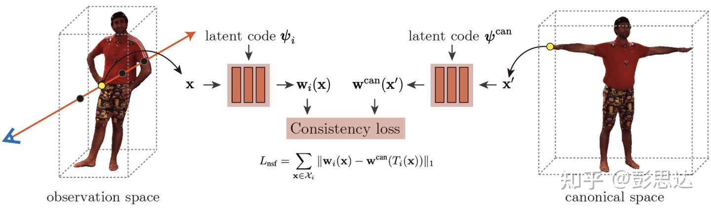
2 形变场/神经混合权重场 Neural blend weight field
2.1 线性蒙皮模型 Linear Blend Skinning Model
正则空间中的点 $\mathbf v$ 通过如下关系映射到视频帧:
\[\begin {equation} \mathbf{v}^{\prime}=\left(\sum_{k=1}^{K} w(\mathbf{v})_{k} G_{k}\right) \mathbf{v} \end {equation}\]人体骨骼定义 $K$$w(\mathbf{v}){k}$是第 每个部分对应一个变换矩阵 ${G_k } \in SE(3)$。$w(\mathbf{v}){k}$表示第 $k$ 个部分的混合权重。
类似的,对于一个视频帧中的点,根据该帧定义的混合权重 $w^{o}(\mathbf{x})$,我们可以把它变换到正则空间中
\[\begin {equation} \mathbf{x}^{\prime}=\left(\sum_{k=1}^{K} w^{o}(\mathbf{x})_{k} G_{k}\right)^{-1} \mathbf{x} \end {equation}\]
2.2 蒙皮权重的求解 Obtaining blend weight per frame
如果让网络直接输出蒙皮权重,会容易收敛到局部最小值。为了解决这个问题,我们首先对任意三维点赋予一个初始化的SMPL蒙皮权重,然后用 MLP 网络 $F_{\Delta \mathbf{w}}:\left(\mathbf{x}, \boldsymbol{\psi}{i}\right) \rightarrow \Delta \mathbf{w}{i}$ 预测一个残差值 residual vector($\psi_{i}$ 是每帧通过学习得到的latent code,$\Delta \mathbf{w}_{i}\in \mathbb{R}^{K}$是残差向量),两者相加得到最终的蒙皮权重。
第 $i$ 帧的蒙皮权重场定义为:
\[\begin {equation} \mathbf{w}_{i}(\mathbf{x})=\operatorname{norm}\left(F_{\Delta \mathbf{w}}\left(\mathbf{x}, \boldsymbol{\psi}_{i}\right)+\mathbf{w}^{\mathrm{s}}\left(\mathbf{x}, S_{i}\right)\right) \end {equation}\]${w}^{\mathrm{s}}$ 是基于SMPL模型 $S_i$ 计算出的初始权重,对任意的3D点,首先找到SMPL mesh 表面最近的点,然后在相应的mesh facet上的三个vertex的蒙皮权重使用 barycentric interpolation 计算出对应的 blend weight。$\operatorname{norm}(\mathbf{w})=\mathbf{w} / \sum w_{i}$。
2.3 正则空间的蒙皮权重场 $\mathbf w ^\text{can}$
为了驱动习得的模版 NeRF 场,还需要额外学习正则空间的neural blend weight蒙皮权重场 $\mathbf w ^\text{can}$。这时,SMPL蒙皮权重 $\mathbf w^\text{can}$根据 T-pose SMPL静止状态计算得出,$F_{\Delta \mathbf{w}}$ 需要根据额外的 latent code $\psi ^\text{can}$ 计算。论文通过约束让视频帧坐标系和正则坐标系的对应点的blend weight相同来学习正则空间中的 neural blend weight field。
3 训练
$F_{\sigma}, F_{\mathbf{c}}, F_{\Delta \mathbf{w}},\left{\boldsymbol{\ell}{i}\right}, \left{\boldsymbol{\psi}{i}\right}$通过最小化渲染和gt误差优化:
\[\begin {equation} L_{\mathrm{rgb}}=\sum_{r \in \mathcal{R}}\left\|\tilde{\mathbf{C}}_{i}(\mathbf{r})-\mathbf{C}_{i}(\mathbf{r})\right\|_{2} \end {equation}\]$\mathcal{R}$ 是通过图片像素点的光线集合。
在驱动人体模型时,我们需要优化视频帧坐标系下的neural blend weight field。这个也是通过约束视频帧坐标系和正则坐标系的对应点的blend weight相同来进行训练。需要注意的是,正则坐标系的neural blend weight field在训练新动作的人体模型时参数是固定的。
\[\begin {equation} L_{\mathrm{nsf}}=\sum_{\mathbf{x} \in \mathcal{X}_{i}}\left\|\mathbf{w}_{i}(\mathbf{x})-\mathbf{w}^{\mathrm{can}}\left(T_{i}(\mathbf{x})\right)\right\|_{1} \end {equation}\]$\mathcal{X}_i$ 是第 $i$ 帧 3D bbox内的采样点集合。
训练时上面两个 Loss function 的系数都是 1。
4 驱动 Animation
4.1 新视点合成 Image Synthesis
给定一个新的 pose,首先更新 SMPL pose参数 $S ^ \text{new}$,并且由此计算SMPL蒙皮权重 $\mathbf w_\text{s}$,新的neural blend weight field $\mathbf w^ \text{new}$ 定义为:
\[\begin {equation} \mathbf{w}^{\text {new }}\left(\mathbf{x}, \boldsymbol{\psi}^{\text {new }}\right)=\operatorname{norm}\left(F_{\Delta \mathbf{w}}\left(\mathbf{x}, \boldsymbol{\psi}^{\text {new }}\right)+\mathbf{w}^{\mathrm{s}}\left(\mathbf{x}, S^{\text {new }}\right)\right) \end {equation}\]基于 $\mathbf w ^\text{new}$ 和LBS模型,我们可以产生新的 deformation field 形变场 $T^\text{new}$。需要重新训练的是 latent code $\psi ^ \text{new}$,由下式优化:
\[\begin {equation} L_{\text {new }}=\sum_{\mathbf{x} \in \mathcal{X}^{\text {new }}}\left\|\mathbf{w}^{\text {new }}(\mathbf{x})-\mathbf{w}^{\text {can }}\left(T^{\text {new }}(\mathbf{x})\right)\right\|_{1} \end {equation}\]$\mathcal{X}^\text{new}$ 是新动作下 3D bbox内的采样点集合。注意 $\mathbf{w}^{\text {can }}$ 在训练新动作的人体模型时参数是固定的。
实际上不同动作的skinning field通过改变latent code同时训练。
4.2 3D表面重建 3D shape Generation
类似neural body,把bbox分成voxel,根据 density 值采用 marching cubes 算法提取出 mesh。
新 pose 使用公式(3)转换每个 vertex 位置,产生形变后的mesh。
实现细节
NeRF的 密度场F$\sigma$ 和颜色场 $F\mathbf c$ 和原论文中一样。这里仅仅使用单次采样,每条光线采 64 个点。
$F_{\Delta \mathbf{w}}$ 的结构和上面两个几乎一样,区别是最后一层输出 24 维,此外,对结果应用需要应用 $\text{exp}(·)$。
网络架构
实验结果
近来非常火热的 Neural Implicit Function:
- Volume Rendering based: NeRF 结合poisson surface reconstruction (insufficient surface constraints)
- Surface Rendering based: IDR(require foreground mask as supervision; trapped in local minima; struggle with reconstruction of objects with severe self-occlusion or thin structures)
NeuS 使用 SDF 函数的水平集 (zero-level set of a signed distance function (SDF)) 表示物体的表面,引入SDF导出的密度分布,采用体渲染 volume rendering 训练一个新的神经SDF表示方法。
NeuS 在复杂几何形状和自遮挡情况下都有效,取得了SOTA的效果,重建效果超过 了NeRF 和 IDR,以及同期的 UNISURF。
体渲染可以处理突然的深度变化,但是重建结果的噪声较大。

Related Works
- Traditional multi-view 3D reconstruction
- Point- and surface-based reconstruction methods
- estimate the depth map of each pixel by exploiting inter-image photometric consistency
- then fuse the depth maps into a global dense point cloud
- the surface reconstruction is usually done as a post processing with methods like screened Poisson surface reconstruction
- the reconstruction quality heavily relies on the quality of correspondence matching, and the difficulties in matching correspondence for objects without rich textures often lead to severe artifacts and missing parts in the reconstruction results
- volumetric reconstruction methods
- circumvent the difficulty of explicit correspondence matching by estimating occupancy and color in a voxel grid from multi-view images and evaluating the color consistency of each voxel
- Due to limited achievable voxel resolution, these methods cannot achieve high accuracy
- Point- and surface-based reconstruction methods
- Neural Implicit Representation applications
- shape representation
- novel view synthesis
- multi-view 3D reconstruction
方法
给定物体的照片 ${I_k}$ ,重建物体的表面 $S$。物体表面用signed distance function(SDF)表示,采用MLP编码。
Rendering Procedure
场景表示 Scene Representation
物体形状和颜色分别用SDF场,颜色场函数表示,这两个函数都采用 MLP 编码
- $f: \mathbb{R}^{3} \rightarrow \mathbb{R}$ 把空间点 $\mathbf x \in \mathbb{R}^{3}$ 映射到它距离物体的signed distance
-
物体的表面 $S$ 就用SDF的0-水平集表示:$S = {\mathbf x \in \mathbb{R}^{3} f(\mathbf x)=0}$
-
- $c: \mathbb{R}^{3} \times \mathbb{S}^{2} \rightarrow \mathbb{R}^{3}$ 将空间点的颜色编码成位置 $\mathbf x \in \mathbb{R}^{3}$ 和视角方向 $\mathbf v \in \mathbb{S}^{2}$ 的函数
这里引入概率密度函数 S-density: $\phi(f(\mathbf x))$ ,其中 $\phi_{s}(x)=s e^{-s x} /\left(1+e^{-s x}\right)^{2}$,叫做 logistic density distribution,是 $\Phi_{s}(x)=\left(1+e^{-s x}\right)^{-1}$ 的导数。标准差是 $1/s$,以 0 为对称轴。当网络收敛时,1/s 会逼近0。这里的概率密度函数可以用其他关于0对称的函数替代,这里是为了计算简便。
渲染 Rendering
为了学习 SDF 和 颜色场的MLP参数,采用 volume rendering。
| 给定一个像素点,定义对应的光线 ${ \mathbf p(t) = \mathbf o + t \mathbf v | t \geq 0}$,$\mathbf o$ 是相机中心,$\mathbf v$ 是光线的单位向量,该点的颜色用积分表示为: |
其中, $w(t)$表示空间点 $\mathbf p(t)$ 在观察方向 $\mathbf v$ 的权重,并且满足 $w(t) \geq 0$ 且 $\int_{0}^{+\infty} w(t) \mathrm d t =1$ 。
权重函数 weight function
训练出准确的SDF表达的关键就在于通过SDF函数 $f$ 得到合适的权重函数 $w(t)$ ,$w(t)$有如下要求:
- Unbiased: $w(t)$ 需要在相机光线与物体表面相交点 $\mathbf p (t^)$ (即 $f(\mathbf p (t^))=0$)达到局部最大值。即表面附近的点对最终结果的贡献最大
- Occlusion-aware: 当两个点有同样的SDF值的时候,靠近相机的点的权重应该更大。即当经过多个表面时,最靠近的表面影响最大
根据NeRF中标准的体渲染公式,权重公式定义为:
\[w(t)=T(t) \sigma(t), \quad \text{where} \ T(t) = \exp \left(-\int_{0}^{t} \sigma(u) d u\right)\]$\sigma(t)$ 是 volume density 体密度,$T(t)$ 是accumulated transmittance 累积透射比,表示这一段没有击中任何粒子的概率。
Naive Solution
现在最简单的想法是把 $\sigma (t)$ 设为S-density,即 $\sigma (t) = \phi(f(\mathbf p(t)))$。虽然是 occlusion-aware 的,但$w(t)$ 在光线到达交界点之前就达到了局部最大。

Our Solution
首先介绍直接把normalized S-density 作为权重的方法,这种方法满足unbiased,但是无法处理穿过多个表面的情况。
\[w(t)=\frac{\phi_{s}(f(\mathbf{p}(t)))}{\int_{0}^{+\infty} \phi_{s}(f(\mathbf{p}(u))) \mathrm{d} u}\]仿照体渲染公式,定义 opaque density function $\rho(t)$,代替标准体渲染中的 $\sigma$。权重方程表示为:
\[w(t)=T(t) \rho(t), \quad \text { where } T(t)=\exp \left(-\int_{0}^{t} \rho(u) \mathrm{d} u\right)\]| 根据几何关系,$f(\mathbf p (t)) = | \cos (\theta) | \cdot\left(t-t^{}\right)$,其中$f(\mathbf p (t^))=0$,$\theta$ 是视角方向与物体表面法向量 $\mathbf n$ 的夹脚,这里可以看成常量。仍然使用上面的直接方法表示权重$w(t)$,有 |
| 为了求出 $\rho(t)$,有 $T(t) \rho(t) = | \cos (\theta) | \phi_{s}(f(\mathbf{p}(t))) = -\frac{\mathrm{d} \Phi_{s}}{\mathrm{~d} t}(f(\mathbf{p}(t))) = \frac {\mathrm{d}T}{\mathrm{d}t}(t)$ |
所以,$T(t)=\Phi_{s}(f(\mathbf{p}(t)))$,求得
\[\rho(t)=\frac{-\frac{\mathrm{d} \Phi_{s}}{\mathrm{~d} t}(f(\mathbf{p}(t)))}{\Phi_{s}(f(\mathbf{p}(t)))}\]上式是单个surface的情况,当光线在两个surface之间时会变成负,把它拓展到多surface的情况需要在这时将之设为0。
\[\rho(t)=\max \left(\frac{-\frac{\mathrm{d} \Phi_{s}}{\mathrm{~d} t}(f(\mathbf{p}(t)))}{\Phi_{s}(f(\mathbf{p}(t)))}, 0\right)\]最后再使用 $w(t)=T(t) \rho(t)$ 计算出权重方程。

Discretization
类似 NeRF,定义采样点 $n$ 个:$\left{\mathbf{p}{i}=\mathbf{o}+t{i} \mathbf{v} \mid i=1, \ldots, n, t_{i}<t_{i+1}\right}$,计算的像素颜色为:
\[\hat{C}=\sum_{i=1}^{n} T_{i} \alpha_{i} c_{i}\]- $T_{i}=\prod_{j=1}^{i-1}\left(1-\alpha_{j}\right)$ 是离散的累积透射比accumulated transmittance。
- $\alpha_{i}=1-\exp \left(-\int_{t_{i}}^{t_{i+1}} \rho(t) \mathrm{d} t\right)$ 是离散的浑浊度 opacity value。
$\alpha_i$ 对应前面提到的$\rho$,可以进一步表示为:
\[\alpha_{i}=\max \left(\frac{\Phi_{s}\left(f\left(\mathbf{p}\left(t_{i}\right)\right)-\Phi_{s}\left(f\left(\mathbf{p}\left(t_{i+1}\right)\right)\right)\right.}{\Phi_{s}\left(f\left(\mathbf{p}\left(t_{i}\right)\right)\right)}, 0\right)\]Training
分为有mask和无mask两种情况。为了优化网络和标准差倒数$s$,随机采样一个batch的像素点和对应的光线$P=\left{C_{k}, M_{k}, \mathbf{O}{k}, \mathbf{v}{k}\right}$,$C_k$ 是像素点颜色,$M_k \in {0,1}$ 指是否存在mask。batch大小设为$m$,一条光线上的采样点数设为 $n$。
定义损失函数:
\[\mathcal{L}=\mathcal{L}_{\text {color }}+\lambda \mathcal{L}_{\text {reg }}+\beta \mathcal{L}_{\text {mask }}\]| 其中,$\mathcal{L}{\text {color }}=\frac{1}{m} \sum{k} \mathcal{R}\left(\hat{C}{k}, C{k}\right)$,类似IDR,$\mathcal{R}$ 采用 L1 loss;Eikonal 项 $\mathcal{L}{r e g}=\frac{1}{n m} \sum{k, i}\left(\left | \nabla f\left(\hat{\mathbf{p}}_{k, i}\right)\right | -1\right)^{2}$;可选项 $\mathcal{L}{\text {mask }}=\mathrm{BCE}\left(M{k}, \hat{O}{k}\right)$,$\hat{O}{k}=\sum_{i=1}^{n} T_{k, i} \alpha_{k, i}$是采样点权重的和,BCE是 Binary Entropy Loss。 |
分层采样 Hierarchical Sampling
不像NeRF同时优化 coarse 和 fine 网络,这里只维持一个网络,coarse阶段采样的概率是基于 S-density $\phi_s(f(\mathbf x))$ 和一个大的固定的标准差计算得到,而fine阶段采样的概率基于 $\phi_s(f(\mathbf x))$ 和学得的标准差。
实现细节

实验
Surface reconstruction with mask

Surface reconstruction w/o mask

Ablation study

Thin structures

Shree K. Nayar Columbia University https://fpcv.cs.columbia.edu
Linear Camera Model
Forward Imaging Model: 3D to 2D

World Coord → Camera Coord: Coordinate Transformation Camera Coord → Image Coord: Perspective Projection

Perspective Projection
由Forward Imaging model不难发现:
\[\begin{aligned} &\frac{x_{i}}{f}=\frac{x_{c}}{z_{c}} \quad \text { and } \quad \frac{y_{i}}{f}=\frac{y_{c}}{z_{c}} \\ &x_{i}=f \frac{x_{c}}{z_{c}} \quad \text { and } \quad y_{i}=f \frac{y_{c}}{z_{c}} \end{aligned}\]Image Plane
像平面是由感光元件组成的一个个pixel形成的,下面是像平面原点在中心的情况。
$(f_x, f_y)=(m_xf, m_yf)$ 称为 $x$ 和 $y$ 方向的以像素为单位的焦距

通常,像平面的原点并不在中心。

perspective projection equation:
Note: it’s a Non-Linear equation
\[u=f_x\frac{x_c}{z_c}+o_x \quad v=f_y\frac{y_c}{z_c}+o_y\]Camera’s internal geometry is represented by Intrinsic parameters of the camera: $(f_x, f_y,o_x,o_y)$
Homogeneous Coordinates
Linear Model(Intrinsic Matrix) for Perspective Projection:
\[\left[\begin{array}{l} u \\ v \\ 1 \end{array}\right] =\left[\begin{array}{c} f_{x} x_{c}+z_{c} o_{x} \\ f_{y} y_{c}+z_{c} o_{y} \\ z_{c} \end{array}\right]=\left[\begin{array}{cccc} f_{x} & 0 & o_{x} & 0 \\ 0 & f_{y} & o_{y} & 0 \\ 0 & 0 & 1 & 0 \end{array}\right]\left[\begin{array}{c} x_{c} \\ y_{c} \\ z_{c} \\ 1 \end{array}\right]\]Calibration Matrix — Upper Right Triangular Matrix
\[K = \left[\begin{array}{cccc} f_{x} & 0 & o_{x} \\ 0 & f_{y} & o_{y} \\ 0 & 0 & 1 \end{array}\right]\]Intrinsic Matrix
\[M_{int}=[K|0]=\left[\begin{array}{cccc} f_{x} & 0 & o_{x} & 0 \\ 0 & f_{y} & o_{y} & 0 \\ 0 & 0 & 1 & 0 \end{array}\right]\]World-to-Camera Transformation

Extrinsic Parameters
Camera’s Extrinsic Parameters$(R, c_w)$: Camera Position $c_w$ and Camera Orientation(Rotation) $R$ in the World Coordinate frame $\mathcal W$

Orientation/Rotation Matrix $R$ is Orthonormal Matrix

World-to-Camera equation:
Homogeneous Coordinates
\[\tilde{\mathbf{x}}_{c}=\left[\begin{array}{c}x_{c} \\ y_{c} \\ z_{c} \\ 1\end{array}\right]=\left[\begin{array}{cccc}r_{11} & r_{12} & r_{13} & t_{x} \\ r_{21} & r_{22} & r_{23} & t_{y} \\ r_{31} & r_{32} & r_{33} & t_{z} \\ 0 & 0 & 0 & 1\end{array}\right]\left[\begin{array}{c}x_{w} \\ y_{w} \\ z_{w} \\ 1\end{array}\right]\] \[\tilde{\mathbf{x}}_{c}=M_{\text {ext }} \tilde{\mathbf{x}}_{w}\]Extrinsic Matrix:
\[M_{e x t}=\left[\begin{array}{ll} R_{3 \times 3} & \mathbf{t} \\ \mathbf{0}_{1 \times 3} & 1 \end{array}\right]=\left[\begin{array}{cccc} r_{11} & r_{12} & r_{13} & t_{x} \\ r_{21} & r_{22} & r_{23} & t_{y} \\ r_{31} & r_{32} & r_{33} & t_{z} \\ 0 & 0 & 0 & 1 \end{array}\right]\]Projection Matrix $P$
Combining the $M_{int}$ and $M_{ext}$, we get the full projection matrix P:
\[\widetilde{\mathbf{u}}=M_{\text {int }} M_{\text {ext }} \tilde{\mathbf{x}}_{\boldsymbol{w}}=P \tilde{\mathbf{x}}_{\boldsymbol{w}}\] \[\left[\begin{array}{c}\tilde{u} \\ \tilde{v} \\ \tilde{W}\end{array}\right]=\left[\begin{array}{llll}p_{11} & p_{12} & p_{13} & p_{14} \\ p_{21} & p_{22} & p_{23} & p_{24} \\ p_{31} & p_{32} & p_{33} & p_{34}\end{array}\right]\left[\begin{array}{c}x_{w} \\ y_{w} \\ z_{w} \\ 1\end{array}\right]\]Camera Calibration
“Method to find a camera’s internal and external parameters”(estimate the projection matrix)
- Step1: Capture an image of an object with known geometry
- place world coord frame at one corner of the cube
- take a single image of the cube

- Step2: Identify correspondences between 3D scene points and image points
- Step3: For each corresponding point $i$ in scene and image, we establish a projection equation
- Step4: Rearranging the terms
- Step5: Solve for $\mathbf P$: $AP =0$
- Note: Projection Matrix $P$ is defined only up to a scale. So we can set projection matrix to arbitrary scale
- Actually, we set scale so that $\left| \mathbf p\right|^2 = 1$

We want $A\mathbf p$ as close to 0 as possible and $\left| \mathbf p\right|^2 = 1$:
\[\min _{\mathbf{p}}\|A \mathbf{p}\|^{2}\quad \text{such that}\quad \|\mathbf{p}\|^{2}=1 \\ \min _{\mathbf{p}}\left(\mathbf{p}^{T} A^{T} A \mathbf{p}\right) \quad\text{such that} \quad\mathbf{p}^{T} \mathbf{p}=1\]Define Loss function $L(\mathbf p, \lambda)$:
\[L(\mathbf{p}, \lambda)=\mathbf{p}^{T} A^{T} A \mathbf{p}-\lambda\left(\mathbf{p}^{T} \mathbf{p}-1\right)\]Taking derivatives of $L(\mathbf p, \lambda)$ w.r.t. $\mathbf p$: $2 A^{T} A \mathbf p-2 \lambda\mathbf p=0$
\[A^{T} A \mathbf p =\lambda\mathbf p\]This is the Eigenvalue Problem. Eigenvector with smallest eigenvalue $\lambda$ of matrix $A^{T} A$ minimizes the loss function $L(\mathbf p)$
Then we rearrange solution $\mathbf p$ to form the projection matrix $P$
Extracting Intrinsic and Extrinsic Matrices (from Projection Matrix)


Simple/Calibrated Stereo (Horizontal Stereo)
Triangulation using two cameras

The distance between two cameras is called “Horizontal Baseline”
Solving for $(x,y,z)$:
\[x=\frac{b\left(u_{l}-o_{x}\right)}{\left(u_{l}-u_{r}\right)} \quad y=\frac{b f_{x}\left(v_{l}-o_{y}\right)}{f_{y}\left(u_{l}-u_{r}\right)} \quad z=\frac{bf_x}{\left(u_{l}-u_{r}\right)}\]Where $\left( u_l-u_r\right)$ is called Disparity.
- Depth $z$ is inversely proportional to Disparity.
- Disparity is proportional to Baseline.
- larger the baseline, more precise the disparity is.
Stereo Matching: Finding Disparities
Cooresponding scene points must lie on the same horizontal scan line.
-
Determine Disparity using Template Matching.

Similarity Differences for Template Matching

Issues with Stereo Matching
- Surface must have non-repetitive texture(pattern)
- Foreshortening effects makes matching challenging
Window Size

Uncalibrated Stereo
“Method to estimate/recover 3D structure of a static scene from two arbitrary views”
Assume that:
- Intrinsics $(f_x, f_y, o_x, o_y)$ are known for both views/cameras.
- Extrinsics (relative position/orientation of cameras) are unknown.

Procedure:
- Assume Camera Matrix $K$ is known for each camera
- Find a few/set of Reliable Corresponding Points/Features
- Find Relative Camera Position $\mathrm{t}$ and Orientation $R$
- Find Dense Correspondence ( e.g. using SIFT or hand-picked )
- Compute Depth using Triangulation
Epipolar Geometry

- Epipoles: Image point of origin/pinhole of one camera as viewed by the other camera.
- $\mathbf{e} {l}$ *and $\mathbf{e}{r}$* are the epipoles.
- $\mathbf{e}_{l}$ and $\mathbf{e}_{r}$ are unique for a given stereo pair.
- Epipolar Plane of Scene Point $P$ : The plane formed by camera origins $\left(O_{l}\right.$ , $\left.O_{r}\right)$, epipoles $\left(\mathbf{e}{l}\right. , \left.\mathbf{e}{r}\right)$ and scene point $P$.
- Every scene point lies on a unique epipolar plane.
- Epipolar Constraint: Vector normal to the epipolar plane: $\mathbf n=t\times \mathbf{x}_{l}$
- $\mathbf{x}{l} \cdot\left(\mathrm{t} \times \mathbf{x}{l}\right)=0$
Esssential Matrix
Definition
-
Derivation
From the epipolar constraint:
\[\begin{aligned} &\left[\begin{array}{lll} x_{l} & y_{l} & z_{l} \end{array}\right]\left[\begin{array}{l} t_{y} z_{l}-\iota_{z} y_{l} \\ t_{z} x_{l}-t_{x} z_{l} \\ t_{x} y_{l}-t_{y} x_{l} \end{array}\right]=0 \quad \text { Cross-product definition }\\ &\left[\begin{array}{lll} x_{l} & y_{l} & z_{l} \end{array}\right]\left[\begin{array}{ccc} 0 & -t_{z} & t_{y} \\ t_{z} & 0 & -t_{x} \\ -t_{y} & t_{x} & 0 \end{array}\right]\left[\begin{array}{l} x_{l} \\ y_{l} \\ z_{l} \end{array}\right]=0 \quad \text { Matrix-vector form } \end{aligned}\]$\mathbf{t}{3 \times 1}$ **: Position of Right Camera in Left Camera’s Frame *$R{3 \times 3}$* : Orientation of Left Camera in Right Camera’s Frame
\[\mathbf{x}_{l}=R \mathbf{x}_{r}+\mathbf{t} \quad\left[\begin{array}{l} x_{l} \\ y_{l} \\ z_{l} \end{array}\right]=\left[\begin{array}{lll} r_{11} & r_{12} & r_{13} \\ r_{21} & r_{22} & r_{23} \\ r_{31} & r_{32} & r_{33} \end{array}\right]\left[\begin{array}{l} x_{r} \\ y_{r} \\ z_{r} \end{array}\right]+\left[\begin{array}{l} t_{x} \\ t_{y} \\ t_{z} \end{array}\right]\]Substituting into the epipolar constraint gives:
\[\left[\begin{array}{lll} x_{l} & y_{l} & z_{l} \end{array}\right]\left(\left[\begin{array}{ccc} 0 & -t_{z} & t_{y} \\ t_{z} & 0 & -t_{x} \\ -t_{y} & t_{x} & 0 \end{array}\right]\left[\begin{array}{lll} r_{11} & r_{12} & r_{13} \\ r_{21} & r_{22} & r_{23} \\ r_{31} & r_{32} & r_{33} \end{array}\right]\left[\begin{array}{l} x_{r} \\ y_{r} \\ z_{r} \end{array}\right]+\left[\begin{array}{ccc} 0 & -t_{z} & t_{y} \\ t_{z} & 0 & -t_{x} \\ -t_{y} & t_{x} & 0 \end{array}\right]\left[\begin{array}{l} t_{x} \\ t_{y} \\ t_{z} \end{array}\right]\right)=0\]Cause: $\mathbf t \times \mathbf t =0$, we have:
\[\left[\begin{array}{lll} x_{l} & y_{l} & z_{l} \end{array}\right]\left[\begin{array}{lll} e_{11} & e_{12} & e_{13} \\ e_{21} & e_{22} & e_{23} \\ e_{31} & e_{32} & e_{33} \end{array}\right]\left[\begin{array}{l} x_{r} \\ y_{r} \\ z_{r} \end{array}\right]=0\]
Given that $T_{\times}$is a Skew-Symmetric matrix $\left(a_{i j}=-a_{j i}\right)$ and $R$ is an Orthonormal matrix, it is possible to “decouple” $T_{\times}$ and $R$ from their product using “Singular Value Decomposition”.
- If $E$ is known, we can calculate $\mathbf t$ and $R$
How to get Essential Matrix ?
We don’t have $\mathbf x_l$ (3D position in left camera coordinates) and $\mathbf x_r$, we do know cooresponding points in image coordinates.
Fundamental Matrix
-
Derivation:
Perspective projection equations for left camera:
\[\begin{aligned} u_{l} &=f_{x}^{(l)} \frac{x_{l}}{z_{l}}+o_{x}^{(l)} & v_{l} &=f_{y}^{(l)} \frac{y_{l}}{z_{l}}+o_{y}^{(l)} \\ z_{l} u_{l} &=f_{x}^{(l)} x_{l}+z_{l} o_{x}^{(l)} & z_{l} v_{l} &=f_{y}^{(l)} y_{l}+z_{l} o_{y}^{(l)} \end{aligned}\]In matrix form:
\[Z_{l}\left[\begin{array}{c} u_{l} \\ v_{l} \\ 1 \end{array}\right]=\left[\begin{array}{c} Z_{l} u_{l} \\ Z_{l} v_{l} \\ Z_{l} \end{array}\right]=\left[\begin{array}{ccc} f_{x}^{(l)} x_{l}+Z_{l} o_{x}^{(l)} \\ f_{y}^{(l)} y_{l}+Z_{l} o_{y}^{(l)} \\ Z_{l} \end{array}\right]=\left[\begin{array}{ccc} f_{x}^{(l)} & 0 & o_{x}^{(l)} \\ 0 & f_{y}^{(l)} & o_{y}^{(l)} \\ 0 & 0 & 1 \end{array}\right]\left[\begin{array}{l} x_{l} \\ y_{l} \\ z_{l} \end{array}\right]\] \[\begin{aligned} \text{Left camera}\quad&\mathbf{x}_{l}^{T}=\left[\begin{array}{lll} u_{l} & v_{l} & 1 \end{array}\right] z_{l} {K_{l}^{-1}}^{T}\\ &\text{Right camera}\quad\mathbf{x}_{r}=K_{r}^{-1} z_{r}\left[\begin{array}{c} u_{r} \\ v_{r} \\ 1 \end{array}\right] \end{aligned}\]Rewrite epipolar constraint:
\[\left[\begin{array}{lll} u_{l} & v_{l} & 1 \end{array}\right] z_{l} {K_{l}^{-1}}^T\left[\begin{array}{lll} e_{11} & e_{12} & e_{13} \\ e_{21} & e_{22} & e_{23} \\ e_{31} & e_{32} & e_{33} \end{array}\right] K_{r}^{-1} z_{r}\left[\begin{array}{c} u_{r} \\ v_{r} \\ 1 \end{array}\right]=0\]And $z_l, z_r ≠ 0$
\[\left[\begin{array}{lll} u_{l} & v_{l} & 1 \end{array}\right]{K_{l}^{-1}}^T\left[\begin{array}{lll} e_{11} & e_{12} & e_{13} \\ e_{21} & e_{22} & e_{23} \\ e_{31} & e_{32} & e_{33} \end{array}\right] K_{r}^{-1} \left[\begin{array}{c} u_{r} \\ v_{r} \\ 1 \end{array}\right]=0\]
Definition
\[\left[\begin{array}{lll} u_{l} & v_{l} & 1 \end{array}\right]\left[\begin{array}{lll} f_{11} & f_{12} & f_{13} \\ f_{21} & f_{22} & f_{23} \\ f_{31} & f_{32} & f_{33} \end{array}\right]\left[\begin{array}{c} u_{r} \\ v_{r} \\ 1 \end{array}\right]=0\] \[E=K_{l}^{T} F K_{r}\]Estimating Fundamental Matrix and T, R
-
For each coorespondence i, write out the epipolar constraint:
\[\left[\begin{array}{lll} u_{l} & v_{l} & 1 \end{array}\right]\left[\begin{array}{lll} f_{11} & f_{12} & f_{13} \\ f_{21} & f_{22} & f_{23} \\ f_{31} & f_{32} & f_{33} \end{array}\right]\left[\begin{array}{c} u_{r} \\ v_{r} \\ 1 \end{array}\right]=0\]then expand the matrix to get linear equation
-
Rearrange the terms to form a linear system: $A \mathbf f = 0$

-
Find least squares solution for fundamental matrix $F$. Fundamental matrix acts on homogeneous coordinates. Set fundamental matrix to some arbitrary scale. then rearrange solution $\mathbf f$ to get form the fundamental matrix F
- Compute essential matrix $E$ from known left and right intrinsic camera matrices and fundamental matrix $F$.
- Extract $R$ and $\mathbf{t}$ from $E$.(Using Singular Value Decomposition)
Finding Coorespondences

- Epipolar Line: Intersection of image plane and epiplar plane ( e.g. $\mathbf u_l \mathbf e_l$ and $\mathbf u_r \mathbf e_r$ )
- Given a point in one image, the corresponding point in the other image must lie on the epipolar line.
- Finding correspondence reduces to a 1D search.
Finding Epipolar Lines

Computing Depth using Triangulation
Left Camera Imaging Equation:
\[\begin{gathered} {\left[\begin{array}{c} u_{l} \\ v_{l} \\ 1 \end{array}\right] \equiv\left[\begin{array}{cccc} f_{x}^{(l)} & 0 & o_{x}^{(l)} & 0 \\ 0 & f_{y}^{(l)} & o_{y}^{(l)} & 0 \\ 0 & 0 & 1 & 0 \end{array}\right]\left[\begin{array}{cccc} r_{11} & r_{12} & r_{13} & t_{x} \\ r_{21} & r_{22} & r_{23} & t_{y} \\ r_{31} & r_{32} & r_{33} & t_{z} \\ 0 & 0 & 0 & 1 \end{array}\right]\left[\begin{array}{c} x_{r} \\ y_{r} \\ z_{r} \\ 1 \end{array}\right]} \\ \tilde{\mathbf{u}_{\boldsymbol{l}}}=P_{l} \tilde{\mathbf{x}}_{\boldsymbol{r}} \end{gathered}\]Right Camera Imaging Equation:
\[\begin{gathered} {\left[\begin{array}{c} u{r} \\ v_{r} \\ 1 \end{array}\right] \equiv\left[\begin{array}{cccc} f_{x}^{(r)} & 0 & o_{x}^{(r)} & 0 \\ 0 & f_{y}^{(r)} & o_{y}^{(r)} & 0 \\ 0 & 0 & 1 & 0 \end{array}\right]\left[\begin{array}{c} x_{r} \\ y_{r} \\ z_{r} \\ 1 \end{array}\right]} \\ \widetilde{\mathbf{u}}_{r}=M_{i n t_{r}} \widetilde{\mathbf{x}}_{r} \end{gathered}\]

Find least squares solution using pseudo-inverse:
\[\begin{gathered} A \mathbf{x}{r}=\mathbf{b} \\ A^{T} A \mathbf{x}{r}=A^{T} \mathbf{b} \\ \mathbf{x}_{r}=\left(A^{T} A\right)^{-1} A^{T} \mathbf{b} \end{gathered}\]Applications:
- 3D reconstruction with Internet Images
-
Active Stereo Results

Stereo Vision in Nature
- Predator eyes are configured for depth estimation
- Prey eyes are configured for larger field of view

论文链接:https://zju3dv.github.io/neuralbody/
Demo:
- 从稀疏视角视频中合成自由视角
- 人物 3D 重建(geometry(extracted from density volumes),appearance)
局限性:
cannot synthesize images of novel human poses as 3D convolution is not equivariant to pose changes
1. Introduction
Problem
生成动态人体的自由视角视频,这有很多应用,包括电影工业,体育直播和远程视频会议,以及实现低成本的子弹时间特效。
Related work
现在效果最好的视角合成方法主要是NeRF 这个方向的论文,但他们有两个问题:
- 需要非常稠密视角来训练视角合成网络。比如NeRF论文中,一般用了100多个视角来训练网络。
- NeRF只能处理静态场景。现在大部分视角合成工作是对于每个静态场景训一个网络,对于动态场景,上百帧需要训上百个网络,这成本很高。
Key Idea
在稀疏视角下,单帧的信息不足以恢复正确的3D scene representation。论文通过视频的整合时序信息来获得足够多的3D shape observation。实际生活中的经验是,观看一个动态的物体更能想象他的三维形状。

这里整合时序信息的实现用的是latent variable model。具体来说,我们定义了一组隐变量,从同一组隐变量中生成不同帧的场景,这样就把不同帧观察到的信息和一组隐变量关联在了一起。经过训练,我们就能把视频各个帧的信息整合到这组隐变量中,也就整合了时序信息。
2. Neural body
NeRF的网络是一个global implicit function。global的意思是NeRF只用一个MLP网络去记录场景中所有点的颜色和几何信息。

Implicit neural representation with structured latent codes
2.1 Structured latent codes
Latent codes的生成:对于某一帧,论文定义了一组离散的 local latent codes 锚定在SMPL人体模型的6890个定点上:
\[\mathcal{Z}=\left\{\boldsymbol{z}{1}, \boldsymbol{z}{2}, \ldots, \boldsymbol{z}_{6890}\right\}\]论文实际使用了浙大三维视觉实验室开源的 EasyMocap **来从多视角图片 $\left{\mathcal{I}{t}^{c} \mid c=1, \ldots, N{c}\right}$ 检测每一帧的SMPL模型参数。
然后我们在可驱动的 SMPL 模型的 mesh vertices上摆放latent codes,这里潜码 $z$ 的维度被设置成 16。
因为这些latent codes可随SMPL模型改变空间位置,从同一组 latent codes 中能生成不同帧的动态人物场景,故称为 structured latent codes。
这组潜码通过一个神经网络,就可以表示局部的几何(geometry)和外貌(appearance(color&density))。
因为所有帧的场景都是通过这一组潜码来生成的,所以不同帧也就自然地被整合起来了。
这里说是 local implicit function 是因为:相比于NeRF用一个MLP记录整个场景的信息,本文场景的信息记录在local latent codes。比如脸部和手部的 latent codes 分别记录脸和手的 appearance 和 shape information。
2.2 Code diffusion
将local latent codes输入到一个3维卷积神经网络 SparseConvNet,得到一个latent code volume,这样就能通过插值得到空间中的任意一点的latent code。
We compute the 3D bounding box of the human and divide the box into small voxels with voxel size of 5mm × 5mm × 5mm. The latent code of a non-empty voxel is the mean of latent codes of SMPL vertices inside this voxel. SparseConvNet utilizes 3D sparse convolutions to process the input volume and output latent code volumes with 2×, 4×, 8×, 16× downsampled sizes. With the convolution and downsampling, the input codes are difused to nearby space. Following [56], for any point in 3D space, we interpolate the latent codes from multi-scale code volumes of network layers 5, 9, 13, 17, and concate- nate them into the final latent code.
Since the code diffusion should not be affected by the human position and orientation in the world coordinate system, we transform the code locations to the SMPL coordinate system.

Architecture of SparseConvNet. Each layer consists of sparse convolution, batch normalization and ReLU.
$\mathbf x$ 首先被转换到 SMPL 坐标系中,然后使用 trilinear interpolation 扩散潜码到空间的任意位置。
将点 $\mathbf x$ 处的latent code表示为:
\[\psi\left(\mathbf{x}, \mathcal{Z}, S_{t}\right)\]2.3 Density and color regression
把潜码 $\psi\left(\mathbf{x}, \mathcal{Z}, S_{t}\right)$ 送入NeRF的网络 (MLP) 中,就能得到相应的 color 和 density。
Density model透明度:
对 t 帧,点 $\mathbf x$ 处的 volume density 是潜码的函数,这里使用4层MLP:
\[\sigma_{t}(\mathbf{x})=M_{\sigma}\left(\psi\left(\mathbf{x}, \mathcal{Z}, S_{t}\right)\right)\]Color model:
为每帧添加了一个 latent embedding $\ell_{t}$,使用2层MLP,$\mathbf d$ 表示观察方向。
效法 NeRF 中的 positional encoding,这里也对观察方向和位置进行了位置编码 $\gamma()$ 。
\[\mathbf{c}_{t}(\mathbf{x})=M_{\mathbf{c}}\left(\psi\left(\mathbf{x}, \mathcal{Z}, S_{t}\right), \gamma_{\mathbf{d}}(\mathbf{d}), \gamma_{\mathbf{x}}(\mathbf{x}), \boldsymbol{\ell}_{t}\right)\]2.4 Volume rendering
用于生成不同视角观察到的图片。
第 t 帧,在SMPL模型的近端和远端附近,沿相机光线 $\mathbf c$ 采样 $N_k$ 个点,最后每个像素点渲染出来的颜色 $\tilde{C}_{t}(\mathbf{r})$ 是
\[\begin{gathered} \tilde{C}_{t}(\mathbf{r})=\sum_{k=1}^{N_{k}} T_{k}\left(1-\exp \left(-\sigma_{t}\left(\mathbf{x}_{k}\right) \delta_{k}\right)\right) \mathbf{c}_{t}\left(\mathbf{x}_{k}\right) \\ \text { where } \quad T_{k}=\exp \left(-\sum_{j=1}^{k-1} \sigma_{t}\left(\mathbf{x}_{j}\right) \delta_{j}\right) \end{gathered}\]其中,$\delta_{k}=\left|\mathbf{x}{k+1}-\mathbf{x}{k}\right|_2$ 是相邻两个采样点之间的距离。在实验中,$N_k$ 被设置成 64。
2.5 Training
我们通过最小化体渲染出来的图片和真实图片的差异优化 neural body。
\[minimize \sum_{t=1}^{N_{t}} \sum_{c=1}^{N_{c}} L\left(\mathcal{I}_{t}^{c}, P^{c} ; \ell_{t}, \mathcal{Z}, \Theta\right)\]其中 $\Theta$ 表示网络参数;$P^{c}$ 是相机参数;$L$ 是渲染出来图片和真实图片之间的 total square error,对应的损失函数是:
\[L=\sum_{\mathbf{r} \in \mathcal{R}}\|\tilde{C}(\mathbf{r})-C(\mathbf{r})\|_{2}^{2}\]像NeRF一样,论文用 volume rendering 从图片中优化网络参数。通过在整段视频上训练,Neural Body实现了时序信息的整合。
2.6 Applications
训练完成后的neural body既可以用来合成新视角,也可以用于三维重建。
三维重建的具体方法是:首先将场景离散成一个个 $5mm × 5mm × 5mm$ 的体素,然后算出所有体素的 volume density 体密度,并且使用 Marching Cubes 算法提取出人体的mesh。
3 Experiments
3.1 Novel view synthesis


3.2 3D reconstruction

