| CARVIEW |
 and
and  respectively. The goal of this post is to understand the Sylow
  -subgroups of in more detail and see what we can learn from them about Sylow subgroups in general.
Explicit Sylow theory for
Our starting point is the following.
Baby Lie-Kolchin: Let 


Proof. If 


Now we can argue as follows. If 


Continuing in this way we get a sequence 


Conjugating back to the standard basis, we’ve proven:
Proposition: Every 
This is almost a proof of Sylow I and II for
We can show that it’s Sylow by explicitly dividing its order into the order of 

Claim: The normalizer of 


Corollary (Explicit Sylow I and II for
Proof. The normalizer 


This quotient is the complete flag variety: it can be identified with the action of 

is exactly 
But this is clear: given a complete flag

we can consider the subgroup of 


(This argument works over any field.)
From here it’s not hard to also prove
Explicit Sylow III for 

Proof. Actually we can compute 
![\displaystyle n_p = [n]_p! = \prod_{i=1}^n [i]_p = \prod_{i=1}^n \left( p^{i-1} + p^{i-2} + \dots + 1 \right)](https://s0.wp.com/latex.php?latex=%5Cdisplaystyle+n_p+%3D+%5Bn%5D_p%21+%3D+%5Cprod_%7Bi%3D1%7D%5En+%5Bi%5D_p+%3D+%5Cprod_%7Bi%3D1%7D%5En+%5Cleft%28+p%5E%7Bi-1%7D+%2B+p%5E%7Bi-2%7D+%2B+%5Cdots+%2B+1+%5Cright%29&bg=ffffff&fg=333333&s=0&c=20201002)
which is clearly congruent to
We could also have done this by dividing the order of
![\displaystyle |GL_n(\mathbb{F}_p)| = p^{ {n \choose 2} } (p - 1)^n [n]_p!](https://s0.wp.com/latex.php?latex=%5Cdisplaystyle+%7CGL_n%28%5Cmathbb%7BF%7D_p%29%7C+%3D+p%5E%7B+%7Bn+%5Cchoose+2%7D+%7D+%28p+-+1%29%5En+%5Bn%5D_p%21&bg=ffffff&fg=333333&s=0&c=20201002)
for the order of 
What is going on in these proofs?
Let’s take a step back and compare these explicit proofs of the Sylow theorems for 
. By the PGFPT this means any
.
- The stabilizers of the action of
In fact finding a transitive such action is exactly equivalent to finding a Sylow 

In the explicit proof for 


The next question we’ll address in Part III is: can we do something similar for 
The 
There will be some occasional historical notes taken from Waterhouse’s The Early Proofs of Sylow’s Theorem.
A quick note on the definition of a Sylow subgroup
A Sylow 


So for the rest of this post, a Sylow
Warmup: Cauchy’s theorem
We’ll start off by giving some proofs of Cauchy’s theorem. One of the proofs of Sylow I later needs it as a lemma, and some of the proofs we give here will generalize to proofs of Sylow I. First we quote the proof using the PGFPT in full from the above blog post, as Proof 1.
Cauchy’s theorem: Let
Proof 1 (PGFPT). 

since if 


This proof is almost disgustingly short. By contrast, according to Waterhouse, Cauchy’s original proof runs nine pages (!) and works as follows.
First Cauchy explicitly constructs Sylow 


and the exponent is Legendre’s formula for the largest power 

Second, Cauchy proves a special case of the following lemma, namely the special case that 
Cauchy’s 

Proof. We’ll prove the contrapositive: if
Consider the left action of 
![\displaystyle |H/P| = \sum_{[h] \in G \backslash H/P} \frac{|G|}{|\text{Stab}_G(hP)|}](https://s0.wp.com/latex.php?latex=%5Cdisplaystyle+%7CH%2FP%7C+%3D+%5Csum_%7B%5Bh%5D+%5Cin+G+%5Cbackslash+H%2FP%7D+%5Cfrac%7B%7CG%7C%7D%7B%7C%5Ctext%7BStab%7D_G%28hP%29%7C%7D&bg=ffffff&fg=333333&s=0&c=20201002)
where 

and in particular it has order dividing 
If

and in particular that 
Call a collection of finite groups cofinal if every finite group embeds into at least one of them.
Corollary: To prove Cauchy’s theorem for all finite groups, it suffices to find a cofinal collection of finite groups which have Sylow
We can now complete Cauchy’s proof of Cauchy’s theorem.
Proof 2 (symmetric groups). The symmetric groups 
But we don’t have to use the symmetric groups!
Proof 3 (general linear groups). Since the symmetric groups
![\displaystyle |GL_n(\mathbb{F}_p)| = p^{ {n \choose 2} } (p-1)^n [n]_p!](https://s0.wp.com/latex.php?latex=%5Cdisplaystyle+%7CGL_n%28%5Cmathbb%7BF%7D_p%29%7C+%3D+p%5E%7B+%7Bn+%5Cchoose+2%7D+%7D+%28p-1%29%5En+%5Bn%5D_p%21&bg=ffffff&fg=333333&s=0&c=20201002)
where ![[n]_p!](https://s0.wp.com/latex.php?latex=%5Bn%5D_p%21&bg=ffffff&fg=333333&s=0&c=20201002)
Here’s a fourth proof that doesn’t use Cauchy’s lemma and doesn’t require the clever construction of the first proof; Waterhouse says it’s used by Rotman.
Proof 4 (class equation). We induct on the order of
Next, given a finite group

where the sum runs over non-central conjugacy classes. If 


Sylow I
With very little additional effort the above proof of Cauchy’s
Frobenius’
Proof. Consider as before the sum
![\displaystyle |H/P| = \sum_{[h] \in G \backslash H/P} \frac{|G|}{|h^{-1} G h \cap P|}](https://s0.wp.com/latex.php?latex=%5Cdisplaystyle+%7CH%2FP%7C+%3D+%5Csum_%7B%5Bh%5D+%5Cin+G+%5Cbackslash+H%2FP%7D+%5Cfrac%7B%7CG%7C%7D%7B%7Ch%5E%7B-1%7D+G+h+%5Ccap+P%7C%7D&bg=ffffff&fg=333333&s=0&c=20201002)
obtained by considering the orbits of the action of 


Corollary: To prove that Sylow subgroups exist for all finite groups, it suffices to prove that they exist for a cofinal collection of finite groups.
Now we can give two different proofs of Sylow I, as follows.
Sylow I: Every finite group
(Note that with our definitions if 
Proof 1 (symmetric groups). It suffices to prove the existence of Sylow subgroups for the symmetric groups
Proof 2 (general linear groups). It suffices to prove the existence of Sylow
Proof 2 is the first proof of Sylow I given by Serre in his Finite Groups: An Introduction.
I heard a rumor years ago that these proofs existed but didn’t see them; glad that’s finally settled.
The next proof of Sylow I we’ll present is the one that I saw as an undergraduate, in Artin’s Algebra if memory serves. According to Wikipedia it’s due to Wielandt. Serre attributes it to “Miller-Wielandt” and it’s the second proof he gives.
Proof 3 (action on subsets). Write 


(I found this construction very bizarre and unmotivated as an undergraduate. I like it better now, I guess, but I’m still a little mystified.)
Key observation: An element 


This means that the action of
![\displaystyle {|G| \choose p^k} = \sum_{[S]} \frac{|G|}{|\text{Stab}(S)|}](https://s0.wp.com/latex.php?latex=%5Cdisplaystyle+%7B%7CG%7C+%5Cchoose+p%5Ek%7D+%3D+%5Csum_%7B%5BS%5D%7D+%5Cfrac%7B%7CG%7C%7D%7B%7C%5Ctext%7BStab%7D%28S%29%7C%7D&bg=ffffff&fg=333333&s=0&c=20201002)
where the sum runs over a set of orbit representatives.
Lemma: 
Proof. This is a special case of Lucas’ theorem, which we proved using the PGFPT previously.
It follows that 


This proof is tantalizingly similar to the proof of Frobenius’ lemma above; in both cases the key is to write down an action of
We’re not done with proofs of Sylow I! The next proof is due to Frobenius; Waterhouse stresses that its early use of quotients crucially highlighted the importance of working with abstract groups rather than just groups of substitutions as was standard in early group theory. It generalizes the class equation proof of Cauchy’s theorem above.
Proof 4 (class equation). We again induct on the order of
Now, suppose that 


If 
where again the sum runs over non-central conjugacy classes. Since ![[g_i]](https://s0.wp.com/latex.php?latex=%5Bg_i%5D&bg=ffffff&fg=333333&s=0&c=20201002)


This proof is the first one we’ve seen that provides a halfway reasonable algorithm for finding Sylow subgroups, which is lovely (the first three are more or less just raw existence proofs): pass to the quotient by central
We give one final proof. According to Waterhouse, this one is essentially Sylow’s original proof, and it naturally proves an apparently-slightly-stronger result, interpolating between Cauchy’s theorem and Sylow I. It also provides a (different) algorithm for finding Sylow subgroups.
Sylow I+: Every finite group 
(Note that this result is equivalent to Sylow I as usually stated once we know that finite 
Proof 5 (normalizers + PGFPT). We induct on 

Now suppose we’ve found a subgroup 

On the other hand, the fixed points of this action are precisely the cosets 


of
Lemma: If 
If 


where
This proof gives us an algorithm for finding Sylow subgroups by starting with elements of order
Corollary (normalizer criterion): A
It has another corollary we haven’t quite gotten around to proving yet:
Corollary (Sylow = maximal): Sylow
(Before it could have been the case that there were
These are all the proofs of Sylow I that I know or could track down. After having gone through all of them I think I like proof 4 (class equation) and proof 5 (normalizers) the best. Proof 3 (action on subsets) is really too opaque and too specialized; you only learn from it that Sylow subgroups exist and practically nothing else, whereas proof 4 and proof 5 both teach you more about them, including how to find them. I’m sort of amazed it took me over 10 years after I first ran into the Sylow theorems to finally see a version of Sylow’s original proof, and that when I did, I liked it so much better than the first proof I had seen.
Sylow II and III
These will be short.
Sylow II: Let 
Proof 1. Immediate corollary of Frobenius’ lemma.
Proof 2. Consider the action of 

A fixed point of the action of 

Corollary (Sylow = maximal, again): Sylow
(We’ve now proved this result in three different ways!)
Sylow III: Let 


Proof. Since the Sylow
Subproof 1 (action of

and dividing both sides by 
Subproof 2 (action of 

and the conclusion follows.
Theorem 1: Universal lossless compression is impossible. That is, there is no function which takes as input finite strings (over some fixed alphabet) and always produces as output shorter finite strings (over the same alphabet) in such a way that the latter is recoverable from the former.
Supposedly people sometimes claim to be able to do this. It is as impossible as constructing a perpetual motion machine, if not more so, and for much more easily understandable reasons.
Proof. The problem is simply that there are not enough short strings. To be specific, let’s work with just binary strings. There are 

strings of length at most 

Informally, another way to summarize the argument is that it takes
This argument straightforwardly implies that any lossless compression algorithm which makes at least one of its inputs smaller necessarily makes at least one of its inputs larger, and more broadly draws attention to the set of inputs one might actually want to compress in practice. If you want to compress 1000×1000 images – strings of a million pixels – but you only want to compress, say, photos that humans might actually take, this is potentially much smaller than the set of all 1000×1000 images (for example, because most real images have the property that most of the time, a pixel is close in color to its neighbors), and so the theoretical lower bound on how well such images can be compressed might be much better.
More generally, the situation is improved if you have a probability distribution over inputs you want to compress with low entropy and you only want to compress well on average, which allows you to do something like Huffman coding. (This is a generalization because the uniform distribution over a set of size 

What I like about Theorem 1 is that it is both incredibly easy to prove and a surprisingly deep and important fact. Here is, for example, another very important result that is arguably just a corollary of Theorem 1.
Consider what is in some sense the “ultimate” lossless compression scheme, namely, given a binary string of length
The sense in which Kolmogorov compression is the “ultimate” lossless compression scheme is that whatever decompression is, it surely ought to be computable or else we wouldn’t be able to do it (ignoring for the moment that Kolmogorov compression is uncomputable!), and any compression scheme whatsoever (computable or not) which compresses some complicated input string 
So the Kolmogorov complexity of a string is a lower bound, up to an additive constant, on the length of a string that compresses it, according to any compression scheme with a computable decompression function. (Of course you can come up with a silly compression scheme which “memorizes” any fixed string and compresses it arbitrarily small, but the price you pay is that the Kolmogorov complexity of this string is more or less a lower bound on the size of your decompression program, and also there’s no reason this would help you compress anything you actually care about.)
Now, Theorem 1, applied to Kolmogorov compression, implies the following.
Theorem 2: For every
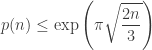
In other words, there exist incompressible strings, whose shortest descriptions are just those strings themselves. In fact, most strings are basically incompressible in this sense; a slight generalization of Theorem 1 shows that at most 


This observation suggests an important connection between incompressibility and randomness. On the one hand, a randomly chosen string is incompressible with high probability. On the other hand, incompressible strings “look random” – they don’t have any patterns in them, because patterns can be described by short programs.
]]>Gradient descent, in its simplest where you just subtract the gradient of your loss function 
This observation can be used to reinvent the learning rate, which, for dimensional consistency, must have units of length squared. It also suggests that the learning rate ought to be set to something like 

It might also make sense to give different parameters different units, which suggests furthermore that one might want a different learning rate for each parameter, or at least that one might want to partition the parameters into different subsets and choose different learning rates for each.
Going much further, from an abstract coordinate-free point of view the extra information you need to compute the gradient of a smooth function is a choice of (pseudo-)Riemannian metric on parameter space, which if you like is a gigantic hyperparameter you can try to optimize. Concretely this amounts to a version of preconditioned gradient descent where you allow yourself to multiply the gradient (in the coordinate-dependent sense) by a symmetric (invertible, ideally positive definite) matrix which is allowed to depend on the parameters. In the first paragraph this matrix was a constant scalar multiple of identity and in the third paragraph this matrix was constant diagonal.
This is an extremely general form of gradient descent, general enough to be equivariant under arbitrary smooth change of coordinates: that is, if you do this form of gradient descent and then apply a diffeomorphism to parameter space, you are still doing this form of gradient descent, with a different metric. For example, if you pick the preconditioning matrix to be the inverse Hessian (in the usual sense, assuming it’s invertible), you recover Newton’s method. This corresponds to choosing the metric at each point to be given by the Hessian (in the usual sense), which is the choice that makes the Hessian (in the coordinate-free sense) equal to the identity. This is a precise version of “the length at which the curvature of
In general it’s expensive to compute the inverse Hessian, so a more practical thing to do is to use a matrix which approximates it in some sense. And now we’re well on the way towards quasi-Newton methods.
]]> over a field . The answer turns out to depend dramatically on whether or not has characteristic zero.
Preliminaries over an arbitrary ring
(All rings and algebras are commutative unless otherwise stated.)
The additive group scheme

This functor is represented by the free ![k[x]](https://s0.wp.com/latex.php?latex=k%5Bx%5D&bg=ffffff&fg=333333&s=0&c=20201002)

and antipode 

A representation of

making it an affine group scheme if 


A representation of
![\mathbb{G}_a \ni x \mapsto \left[ \begin{array}{cc} 1 & x \\ 0 & 1 \end{array} \right]](https://s0.wp.com/latex.php?latex=%5Cmathbb%7BG%7D_a+%5Cni+x+%5Cmapsto+%5Cleft%5B+%5Cbegin%7Barray%7D%7Bcc%7D+1+%26+x+%5C%5C+0+%26+1+%5Cend%7Barray%7D+%5Cright%5D&bg=ffffff&fg=333333&s=0&c=20201002)
which defines a nontrivial action of 
Formally, we can define an action of

such that each 


even though the latter is generally not representable by a scheme, again unless 

The advantage of doing this is that we can appeal to the Yoneda lemma: because
![\text{Aut}_{k[x]}(V \otimes_k k[x]) \subseteq \text{End}_{k[x]}(V \otimes_k k[x]) \cong \text{Hom}_k(V, V \otimes_k k[x])](https://s0.wp.com/latex.php?latex=%5Ctext%7BAut%7D_%7Bk%5Bx%5D%7D%28V+%5Cotimes_k+k%5Bx%5D%29+%5Csubseteq+%5Ctext%7BEnd%7D_%7Bk%5Bx%5D%7D%28V+%5Cotimes_k+k%5Bx%5D%29+%5Ccong+%5Ctext%7BHom%7D_k%28V%2C+V+%5Cotimes_k+k%5Bx%5D%29&bg=ffffff&fg=333333&s=0&c=20201002)
at which point we’ve finally been freed of the burden of having to consider arbitrary ![V \to V \otimes_k k[x]](https://s0.wp.com/latex.php?latex=V+%5Cto+V+%5Cotimes_k+k%5Bx%5D&bg=ffffff&fg=333333&s=0&c=20201002)
![\text{Aut}_{k[x]}(V(k[x]))](https://s0.wp.com/latex.php?latex=%5Ctext%7BAut%7D_%7Bk%5Bx%5D%7D%28V%28k%5Bx%5D%29%29&bg=ffffff&fg=333333&s=0&c=20201002)

Definition-Theorem: A representation of ![\mathcal{O}_{\mathbb{G}_a} \cong k[x]](https://s0.wp.com/latex.php?latex=%5Cmathcal%7BO%7D_%7B%5Cmathbb%7BG%7D_a%7D+%5Ccong+k%5Bx%5D&bg=ffffff&fg=333333&s=0&c=20201002)
This is true more generally for representations of any affine group scheme.
Let’s get somewhat more explicit. A comodule over ![\alpha : V \to V \otimes_k k[x]](https://s0.wp.com/latex.php?latex=%5Calpha+%3A+V+%5Cto+V+%5Cotimes_k+k%5Bx%5D&bg=ffffff&fg=333333&s=0&c=20201002)

which each correspond to an element of 


and the condition that 


as an identity of formal power series, and 3) that for any 


Equating the coefficients of 


from which it follows in particular that the 
Theorem: Over a ring
![\displaystyle k[M_1, M_2, \dots] / \left( {i + j \choose i} M_{i + j} = M_i M_j \right)](https://s0.wp.com/latex.php?latex=%5Cdisplaystyle+k%5BM_1%2C+M_2%2C+%5Cdots%5D+%2F+%5Cleft%28+%7Bi+%2B+j+%5Cchoose+i%7D+M_%7Bi+%2B+j%7D+%3D+M_i+M_j+%5Cright%29&bg=ffffff&fg=333333&s=0&c=20201002)
which are locally finite in the sense that for any
![\displaystyle \sum_i M_i x^i : V \mapsto V \otimes_k k[x]](https://s0.wp.com/latex.php?latex=%5Cdisplaystyle+%5Csum_i+M_i+x%5Ei+%3A+V+%5Cmapsto+V+%5Cotimes_k+k%5Bx%5D&bg=ffffff&fg=333333&s=0&c=20201002)
If 
![(k \otimes \mathbb{Q})[x]](https://s0.wp.com/latex.php?latex=%28k+%5Cotimes+%5Cmathbb%7BQ%7D%29%5Bx%5D&bg=ffffff&fg=333333&s=0&c=20201002)


These representations should really be thought of as continuous representations of the profinite Hopf algebra given as the cofiltered limit over the algebras spanned by 

In characteristic zero
If 

and we conclude the following.
Theorem: Over a 

![\displaystyle \exp (M_1 x) : V \to V \otimes_k k[x]](https://s0.wp.com/latex.php?latex=%5Cdisplaystyle+%5Cexp+%28M_1+x%29+%3A+V+%5Cto+V+%5Cotimes_k+k%5Bx%5D&bg=ffffff&fg=333333&s=0&c=20201002)
The corresponding profinite Hopf algebra is the formal power series algebra ![k[[\partial]]](https://s0.wp.com/latex.php?latex=k%5B%5B%5Cpartial%5D%5D&bg=ffffff&fg=333333&s=0&c=20201002)

Example. The representation ![\left[ \begin{array}{cc} 1 & x \\ 0 & 1 \end{array} \right]](https://s0.wp.com/latex.php?latex=%5Cleft%5B+%5Cbegin%7Barray%7D%7Bcc%7D+1+%26+x+%5C%5C+0+%26+1+%5Cend%7Barray%7D+%5Cright%5D&bg=ffffff&fg=333333&s=0&c=20201002)
![\left[ \begin{array}{cc} 0 & 1 \\ 0 & 0 \end{array} \right]](https://s0.wp.com/latex.php?latex=%5Cleft%5B+%5Cbegin%7Barray%7D%7Bcc%7D+0+%26+1+%5C%5C+0+%26+0+%5Cend%7Barray%7D+%5Cright%5D&bg=ffffff&fg=333333&s=0&c=20201002)
Example. Any coalgebra has a “regular representation,” namely the comodule given by its own comultiplication. The regular representation of
![\displaystyle \mathbb{G}_a \ni x \mapsto (f(y) \mapsto f(y+x)) \in \text{Hom}_k(k[y], k[y] \otimes_k k[x])](https://s0.wp.com/latex.php?latex=%5Cdisplaystyle+%5Cmathbb%7BG%7D_a+%5Cni+x+%5Cmapsto+%28f%28y%29+%5Cmapsto+f%28y%2Bx%29%29+%5Cin+%5Ctext%7BHom%7D_k%28k%5By%5D%2C+k%5By%5D+%5Cotimes_k+k%5Bx%5D%29&bg=ffffff&fg=333333&s=0&c=20201002)
and the corresponding locally nilpotent endomorphism is the derivative 


The regular representation has subrepresentations given by restricting attention to the polynomials of degree at most 
In positive characteristic
In positive characteristic the binomial coefficient 

However, when we try to analyze 


gives by induction

(here we use the fact that we know the 

Continuing from here we find that

using the fact that 


The general situation is as follows. We can write 


Then induction gives

where the LHS is congruent to

This is enough for the
Lemma: Over an
![\displaystyle k[M_1, M_p, \dots]/(M_1^p, M_p^p, \dots)](https://s0.wp.com/latex.php?latex=%5Cdisplaystyle+k%5BM_1%2C+M_p%2C+%5Cdots%5D%2F%28M_1%5Ep%2C+M_p%5Ep%2C+%5Cdots%29&bg=ffffff&fg=333333&s=0&c=20201002)
Corollary: Over an ![k[M_1, M_p, \dots]/(M_1^p, M_p^p, \dots)](https://s0.wp.com/latex.php?latex=k%5BM_1%2C+M_p%2C+%5Cdots%5D%2F%28M_1%5Ep%2C+M_p%5Ep%2C+%5Cdots%29&bg=ffffff&fg=333333&s=0&c=20201002)

![\displaystyle \exp (M_1 x + M_p x^p + \dots) : V \mapsto V \otimes_k k[x]](https://s0.wp.com/latex.php?latex=%5Cdisplaystyle+%5Cexp+%28M_1+x+%2B+M_p+x%5Ep+%2B+%5Cdots%29+%3A+V+%5Cmapsto+V+%5Cotimes_k+k%5Bx%5D&bg=ffffff&fg=333333&s=0&c=20201002)
As before, we can equivalently talk about continuous modules over a suitable profinite Hopf algebra.
Example. We can classify all nontrivial ![J = \left[ \begin{array}{cc} 0 & 1 \\ 0 & 0 \end{array} \right]](https://s0.wp.com/latex.php?latex=J+%3D+%5Cleft%5B+%5Cbegin%7Barray%7D%7Bcc%7D+0+%26+1+%5C%5C+0+%26+0+%5Cend%7Barray%7D+%5Cright%5D&bg=ffffff&fg=333333&s=0&c=20201002)

![\left[ \begin{array}{cc} 0 & c_j \\ 0 & 0 \end{array} \right]](https://s0.wp.com/latex.php?latex=%5Cleft%5B+%5Cbegin%7Barray%7D%7Bcc%7D+0+%26+c_j+%5C%5C+0+%26+0+%5Cend%7Barray%7D+%5Cright%5D&bg=ffffff&fg=333333&s=0&c=20201002)

![\displaystyle \exp \left( J (x^{p^i} + c_{i+1} x^{p^{i+1}} + \dots) \right) = \left[ \begin{array}{cc} 1 & x^{p^i} + c_{i+1} x^{p^{i+1}} + \dots \\ 0 & 1 \end{array} \right]](https://s0.wp.com/latex.php?latex=%5Cdisplaystyle+%5Cexp+%5Cleft%28+J+%28x%5E%7Bp%5Ei%7D+%2B+c_%7Bi%2B1%7D+x%5E%7Bp%5E%7Bi%2B1%7D%7D+%2B+%5Cdots%29+%5Cright%29+%3D+%5Cleft%5B+%5Cbegin%7Barray%7D%7Bcc%7D+1+%26%C2%A0+x%5E%7Bp%5Ei%7D+%2B+c_%7Bi%2B1%7D+x%5E%7Bp%5E%7Bi%2B1%7D%7D+%2B+%5Cdots+%5C%5C+0+%26+1+%5Cend%7Barray%7D+%5Cright%5D&bg=ffffff&fg=333333&s=0&c=20201002)
Contrast to the case of characteristic zero, where there is only one isomorphism class of nontrivial 
Example. Consider again the regular representation given by the translation action of
We find as before that 


we have, over

(for 
(for 
Endomorphisms
Actually we should have expected an answer like this all along, or at least we should have known that we would also need to write down representations involving powers of Frobenius in addition to the obvious representations of the form 


The fact that this sort of thing doesn’t happen in characteristic zero means that
Proposition: Over a ring ![f(x) \in k[x]](https://s0.wp.com/latex.php?latex=f%28x%29+%5Cin+k%5Bx%5D&bg=ffffff&fg=333333&s=0&c=20201002)


Proof. This is mostly a matter of unwinding definitions. By the Yoneda lemma, maps 
![\mathbb{G}_a(k[x]) \cong k[x]](https://s0.wp.com/latex.php?latex=%5Cmathbb%7BG%7D_a%28k%5Bx%5D%29+%5Ccong+k%5Bx%5D&bg=ffffff&fg=333333&s=0&c=20201002)

Now let’s try to classify all such polynomials. Writing 

If 


On the other hand, if 

of powers of the Frobenius map, which is clearly an endomorphism. In summary, we conclude the following.
Proposition: If ![k[F]](https://s0.wp.com/latex.php?latex=k%5BF%5D&bg=ffffff&fg=333333&s=0&c=20201002)

The endomorphisms generated by Frobenius can be used to write down examples of affine group schemes which only exist in positive characteristic. For example, the kernel of Frobenius is the affine group scheme ![\alpha_p \cong \text{Spec } k[x]/x^p](https://s0.wp.com/latex.php?latex=%5Calpha_p+%5Ccong+%5Ctext%7BSpec+%7D+k%5Bx%5D%2Fx%5Ep&bg=ffffff&fg=333333&s=0&c=20201002)

 matrices
  up to change of basis in both the source (
 ) and the target (
 ). In other words, the problem is to describe the equivalence classes of the equivalence relation on matrices given by

It turns out that the equivalence class of 


Continuing in this way, we construct vectors 


Explicitly, this means we can write

where 


Conceptually, the question we’ve asked is: what does a linear transformation 


where 


of a projection onto a direct summand and an inclusion of a direct summand. So the only basis-independent information contained in
The actual problem this blog post is about is more interesting: it is to classify

Conceptually, we’re now asking: what does a linear transformation 
Inventing singular value decomposition
As before, we’ll answer this question by picking bases with respect to which 


as the beginning of an orthonormal basis of 


orthogonal to 


We’ll pick 


At this point we are in trouble unless 
Key lemma #1: Suppose 

Proof. Consider the function

The vectors 


Now we can compute the first-order Taylor series expansion of this function around

so setting the first derivative equal to 
This is the technical heart of singular value decomposition, so it’s worth understanding in some detail. Michael Nielsen has a very nice interactive demo / explanation of this. Geometrically, the points 


Note that this gives a proof that the semiminor axis of an ellipse – the point closest to the origin – is always orthogonal to its semimajor axis. We can think of key lemma #1 above as more or less being equivalent to this fact, also known as the principal axis theorem in the plane, and which is also closely related to but slightly weaker than the spectral theorem for real 
Thanks to key lemma #1, we can continue our construction. With 


where 


The 


This is one version of the singular value decomposition (SVD for short) of 

where 


So, stepping back a bit: what have we learned about what a linear transformation
Looking for more analogies between singular value decomposition and the warmup, we might think of the singular values as a quantitative refinement of the rank, since there are 
Geometrically, one way to describe the answer provided by singular value decomposition to the question “what does a linear transformation look like” is that the key to understanding
Properties
Singular value decomposition has lots of useful properties, some of which we’ll prove here. First, note that taking the transpose of a singular value decomposition 

showing that 
Key lemma #2: Write 


Proof. At the maximum value of 


subject to the above constraints and we already know the solution is given by 
Left-right symmetry: Let 


Proof. Apply key lemma #2 to
Singular = eigen: The left singular vectors 


Proof. We now know that 

and

Hence 

This gives an alternative route to understanding singular value decomposition which comes from writing 

and then applying the spectral theorem to
In addition to the above algebraic characterization of singular values, the singular values also admit the following variational characterization.
Variational characterizations of singular values (Courant, Fischer): We have
and

Proof. For the first characterization, any 

We compute that

and hence that
We conclude that every 

The second characterization is very similar. Any 


We compute that

and hence that

We conclude that every 

The second variational characterization above can be used to prove the following important theorem.
Low rank approximation (Eckart, Young): If 


Proof. Suppose 


and hence that 

The variational characterizations can also be used to prove the following inequality relating the singular values of two matrices and of their sum, which can be thought of as a quantitative refinement of the observation that the rank of a sum 
Additive perturbation (Weyl): Let 


Proof. We want to bound 

To give an upper bound on a minimum value of a function we just need to give an upper bound on some value that it takes. Let 


Since 


The slightly curious off-by-one indexing in the above inequality can be understood as follows: if 


Setting 
Singular values are Lipschitz: The singular values, as functions on matrices, are uniformly Lipschitz with respect to the operator norm with Lipschitz constant

Proof. Apply additive perturbation twice with

(remembering that

(remembering that 
This is very much not the case with eigenvalues: a small perturbation of a square matrix can have a large effect on its eigenvalues. This is explained e.g. in in this blog post by Terence Tao, and is related to pseudospectra.
Setting 

Interlacing: Suppose 

Proof. Apply additive perturbation twice, first to get

and second to get

Interlacing gives us some control over what happens to the singular values under a low-rank perturbation (as opposed to a low-norm perturbation; a low-rank perturbation may have arbitrarily high norm, and vice versa). For example, we learn that if all of the singular values are clumped together, then a rank-
A particular special case of a low-rank perturbation is deleting a small number of rows or columns (note that a row or column which is entirely zero does not affect the singular values, so deleting a row or column is equivalent to setting all of its entries to zero), in which case the upper bound above can be tightened.
Cauchy interlacing: Suppose

Proof. The lower bound follows from interlacing. The upper bound follows from the observation that we have 
Cauchy interlacing also applies to deleting columns, or combinations of rows and columns, because the singular values are unchanged by transposition. In particular, we learn that if
In particular, if all of the singular values of
Three special cases
Three special cases of the general singular value decomposition
First, if 


Second, if 


Finally, if 


is precisely the distance from
In general, we should expect that the SVD of a matrix
be a commutative ring. A popular thing to do on this blog is to think about the Morita 2-category  of algebras, bimodules, and bimodule homomorphisms over , but it might be unclear exactly what we’re doing when we do this. What are we studying when we study the Morita 2-category?
The answer is that we can think of the Morita 2-category as a 2-category of module categories over the symmetric monoidal category 

- objects are the categories
, where
- morphisms are cocontinuous
, and
- 2-morphisms are natural transformations.
An equivalent way to describe the morphisms is that they are “

This action comes from taking the adjoint of the enrichment of
So Morita theory can be thought of as a categorified version of module theory, where we study modules over
Technical preliminaries
Let 


of the homs in 
Thinking of 


All of this terminology has its usual meaning when
The basic analogy
The basic analogy, one piece of structure at a time, goes like this.
- Sets are analogous to categories.
- Abelian groups are analogous to cocomplete categories. (There are several other things we could have said here, but this is the one that’s relevant to thinking about Morita theory. The idea is that taking colimits categorifies addition.)
- Rings are analogous to monoidal cocomplete categories (this includes the condition that the monoidal structure distributes over colimits).
- Commutative rings are analogous to symmetric monoidal cocomplete categories.
- Modules over commutative rings are analogous to cocomplete module categories over symmetric monoidal cocomplete categories.
We won’t get into the generalities of thinking about symmetric monoidal categories or modules over them because, in this post, the only symmetric monoidal categories we care about are those of the form
![\displaystyle \text{Mod}(C) \cong [C^{op}, \text{Mod}(k)]](https://s0.wp.com/latex.php?latex=%5Cdisplaystyle+%5Ctext%7BMod%7D%28C%29+%5Ccong+%5BC%5E%7Bop%7D%2C+%5Ctext%7BMod%7D%28k%29%5D&bg=ffffff&fg=333333&s=0&c=20201002)
on essentially small 

In the special case that the categories
From now on we’ll work in this bigger Morita 2-category, which is now the 2-category deserving the name
- objects essentially small
- morphisms
- 2-morphisms homomorphisms of bimodules.
Equivalently, it has
- objects the cocomplete
(where
- morphisms cocontinuous
- 2-morphisms natural transformations.
From now on, when we say that a
In what ways do the objects of the Morita 2-category behave like modules?
Proposition: The Morita 2-category has biproducts.
In other words, the product 


If 


Proposition: There is a tensor-hom adjunction
![\displaystyle [\text{Mod}(A) \otimes \text{Mod}(B), \text{Mod}(C)] \cong [\text{Mod}(A), [\text{Mod}(B), \text{Mod}(C)]]](https://s0.wp.com/latex.php?latex=%5Cdisplaystyle+%5B%5Ctext%7BMod%7D%28A%29+%5Cotimes+%5Ctext%7BMod%7D%28B%29%2C+%5Ctext%7BMod%7D%28C%29%5D+%5Ccong+%5B%5Ctext%7BMod%7D%28A%29%2C+%5B%5Ctext%7BMod%7D%28B%29%2C+%5Ctext%7BMod%7D%28C%29%5D%5D&bg=ffffff&fg=333333&s=0&c=20201002)
Here the internal hom ![[-, -]](https://s0.wp.com/latex.php?latex=%5B-%2C+-%5D&bg=ffffff&fg=333333&s=0&c=20201002)


(this is a computation, not a definition: the definition is a universal property in terms of functors out of 
Both sides of the equivalence above are equivalent to 

With respect to this tensor product,
Aside: big categories vs. little categories
The biggest secret about category theory that I don’t think is in common circulation is that there are approximately two kinds of categories, and they should be thought of very differently (because the relevant notion of morphism between them is very different):
- Big categories are “categories of mathematical objects.” Typical examples are categories of modules and sheaves. They tend to be cocomplete, and people like to consider cocontinuous functors (really, left adjoints) between them.
- Little categories are “categories as mathematical objects.” Typical examples include categories with one object, or finitely many objects. They tend to be Cauchy complete at best, and people like to consider arbitrary functors, or more generally bimodules, between them.
The Morita 2-categories we discussed above have both little descriptions and big descriptions (via
I think one thing that confuses people when they first start to learn category theory is that the first examples of categories (e.g. groups, rings, modules) tend to be big, even though little categories figure prominently in the theory (e.g. as shapes for diagrams to take limits or colimits over, and/or as things to take presheaves or sheaves on) and feel very different. It’s little categories that can reasonably be thought of as algebraic objects generalizing more familiar objects like monoids and posets (or, in our enriched setting,
On the other hand, the ability to pass between big and little categories is also important. Eilenberg-Watts, as we have seen, gives one version of this: another version is Gabriel-Ulmer duality.
The big vs. little nomenclature suggests, but is not equivalent to, the rigorous distinction between large and small categories, and is related to the distinction between big and little toposes (or, depending on your preferences, between gros and petit topoi) in sheaf theory. The basic point of this distinction is that there are two somewhat different sorts of things people mean by sheaf: on the one hand one might mean a functor on a little category like the category of open subsets of a topological space, and on the other hand one might mean a functor on a big category like the category of commutative rings. It would be nice if people emphasized this distinction more.
Bases, coordinates, and matrices
In terms of higher linear algebra, big categories of modules are “higher vector spaces,” while the little categories that can be used to present the big categories as categories of modules are “bases” for them. As we learned previously, a cocomplete abelian category has a “basis” in this sense iff it has a family of tiny (compact projective) generators, for various notions of generator.
Given a “basis” 

weighted by its “coordinates” 
Similarly, the statement that cocontinuous 
Suppose in particular that 


which deserves to be called the trace of the endomorphism
The identity functor turns out to be represented by 
More explicitly, this coend is the result of coequalizing the left and right actions of
where the two arrows send a pair of morphisms 


By construction, this means that 


for all
Example. Suppose 
![A/[A, A]](https://s0.wp.com/latex.php?latex=A%2F%5BA%2C+A%5D&bg=ffffff&fg=333333&s=0&c=20201002)

The above construction of the trace implies that it is Morita invariant, and 
![\displaystyle \text{tr}(f) \in A/[A, A]](https://s0.wp.com/latex.php?latex=%5Cdisplaystyle+%5Ctext%7Btr%7D%28f%29+%5Cin+A%2F%5BA%2C+A%5D&bg=ffffff&fg=333333&s=0&c=20201002)
This trace is called the Hattori-Stallings trace. For free modules it is computed by taking the image of the sum of the diagonal elements of
In particular, if
The simplest interesting case of the above discussion occurs when 


Higher representation theory
One reason you might want a higher version of linear algebra is to study “higher representation theory,” where groups (or higher versions of groups, such as 2-groups) act on higher vector spaces. Previously we saw such actions occur naturally in Galois descent: namely, if 

More generally, if 


that is, the homotopy fixed point category (which here is typically called “


If the stacky quotient 

Fire
Fire is a sustained chain reaction involving combustion, which is an exothermic reaction in which an oxidant, typically oxygen, oxidizes a fuel, typically a hydrocarbon, to produce products such as carbon dioxide, water, and heat and light. A typical example is the combustion of methane, which looks like

The heat produced by combustion can be used to fuel more combustion, and when that happens enough that no additional energy needs to be added to sustain combustion, you’ve got a fire. To stop a fire, you can remove the fuel (e.g. turning off a gas stove), remove the oxidant (e.g. smothering a fire using a fire blanket), remove the heat (e.g. spraying a fire with water), or remove the combustion reaction itself (e.g. with halon).
Combustion is in some sense the opposite of photosynthesis, an endothermic reaction which takes in light, water, and carbon dioxide and produces hydrocarbons.
It’s tempting to assume that when burning wood, the hydrocarbons that are being combusted are e.g. the cellulose in the wood. It seems, however, that something more complicated happens. When wood is exposed to heat, it undergoes pyrolysis (which, unlike combustion, doesn’t involve oxygen), which converts it to more flammable compounds, such as various gases, and these are what combust in wood fires.
When a wood fire burns for long enough it will lose its flame but continue to smolder, and in particular the wood will continue to glow. Smoldering involves incomplete combustion, which, unlike complete combustion, produces carbon monoxide.
Flames
Flames are the visible parts of a fire. As fires burn, they produce soot (which can refer to some of the products of incomplete combustion or some of the products of pyrolysis), which heats up, producing thermal radiation. This is one of the mechanisms responsible for giving fire its color. It is also how fires warm up their surroundings.
Thermal radiation is produced by the motion of charged particles: anything at positive temperature consists of charged particles moving around, so emits thermal radiation. A more common but arguably less accurate term is black body radiation; this properly refers to the thermal radiation emitted by an object which absorbs all incoming radiation. It’s common to approximate thermal radiation by black body radiation, or by black body radiation times a constant, because it has the useful property that it depends only on the temperature of the black body. Black body radiation happens at all frequencies, with more radiation at higher frequencies at higher temperatures; in particular, the peak frequency is directly proportional to temperature by Wien’s displacement law.
Everyday objects are constantly producing thermal radiation, but most of it is infrared – its wavelength is longer than that of visible light, and so is invisible without special cameras. Fires are hot enough to produce visible light, although they are still producing a lot of infrared light.
Another mechanism giving fire its color is the emission spectra of whatever’s being burned. Unlike black body radiation, emission spectra occur at discrete frequencies; this is caused by electrons producing photons of a particular frequency after transitioning from a higher-energy state to a lower-energy state. These frequencies can be used to detect elements present in a sample in flame tests, and a similar idea (using absorption spectra) is used to determine the composition of the sun and various stars. Emission spectra are also responsible for the color of fireworks and of colored fire.
The characteristic shape of a flame on Earth depends on gravity. As a fire heats up the surrounding air, natural convection occurs: the hot air (which contains, among other things, hot soot) rises, while cool air (which contains oxygen) falls, sustaining the fire and giving flames their characteristic shape. In low gravity, such as on a space station, this no longer occurs; instead, fires are only fed by the diffusion of oxygen, and so burn more slowly and with a spherical shape (since now combustion is only happening at the interface of the fire with the parts of the air containing oxygen; inside the sphere there is presumably no more oxygen to burn):

Black body radiation
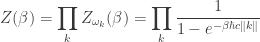
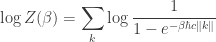
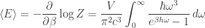
Black body radiation is described by Planck’s law, which is fundamentally quantum mechanical in nature, and which was historically one of the first applications of any form of quantum mechanics. It can be deduced from (quantum) statistical mechanics as follows.
What we’ll actually compute is the distribution of frequencies in a (quantum) gas of photons at some temperature
In statistical mechanics, the probability of finding a system in microstate 

where 


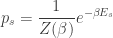
where 
called the partition function. Note that these probabilities don’t change if
It’s a standard observation that the partition function, up to multiplicative scale, contains the same information as the Boltzmann distribution, so anything that can be computed from the Boltzmann distribution can be computed from the partition function. For example, the moments of the energy are given by

and, up to solving the moment problem, this characterizes the Boltzmann distribution. In particular, the average energy is
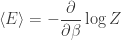
The Boltzmann distribution can be used as a definition of temperature. It correctly suggests that in some sense 
To describe the state of a gas of photons we’ll need to know something about the quantum behavior of photons. In the standard quantization of the electromagnetic field, the electromagnetic field can be treated as a collection of quantum harmonic oscillators each oscillating at various (angular) frequencies 


where 
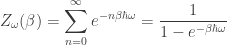
Digression: the (wrong) classical answer
The assumption that 
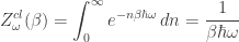
(It’s unclear what measure we should be integrating against here, but but this calculation appears to reproduce the usual classical answer, so I’ll stick with it.)
These two partition functions give very different predictions, although the quantum one approaches the classical one as 
whereas the average energy computed using the classical partition function is
The quantum answer approaches the classical answer as 
The quantum partition function instead predicts that at low frequencies (relative to the temperature) the classical answer is approximately correct, but that at high frequencies the average energy becomes exponentially damped, with more damping at lower temperatures. This is because at high frequencies and low temperatures a quantum harmonic oscillator spends most of its time in its ground state, and cannot easily transition to its next lowest state, which is exponentially less likely. Physicists say that most of this “degree of freedom” (the freedom of an oscillator to oscillate at a particular frequency) gets “frozen out.” The same phenomenon is responsible for classical but incorrect computations of specific heat, e.g. for diatomic gases such as oxygen.
The density of states and Planck’s law
Now that we know what’s going on at a fixed frequency
We’ll make a standard simplifying assumption that our gas of photons is trapped in a box with side length 


and hence (keeping in mind that 


This frequency occurs 

The reason for the simplifying assumptions above are that for a box with periodic boundary conditions (again, mathematically a flat torus) it is very easy to explicitly write down all of the eigenfunctions of the Laplacian: working over the complex numbers for simplicity, they are given by

where 


from which it follows that the multiplicity of a given eigenvalue 

and so the corresponding energy (of a single photon with that frequency) is

At this point we’ll approximate the probability distribution over possible frequencies 


Why is this approximation reasonable (unlike the case of the partition function for a single harmonic oscillator, where it wasn’t)? The full partition function can be described as follows. For each wavenumber 


over all wave numbers
and it is this sum that we want to approximate by an integral. It turns out that for reasonable temperatures and reasonably large boxes, the integrand varies very slowly as
The density of states can be computed as follows. We can think of wave vectors as evenly spaced lattice points living in some “phase space,” from which it follows that the number of wave vectors in some region of phase space is proportional to its volume, at least for regions which are large compared to the lattice spacing 


It remains to compute the volume of the region of phase space given by all wave vectors 


from which we get that the density of states for a single photon is
Actually this formula is off by a factor of two: we forgot to take photon polarization into account (equivalently, photon spin), which doubles the number of states with a given wave number, giving the corrected density
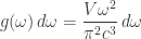
The fact that the density of states is linear in the volume

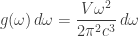
Taking its derivative with respect to
but for us the significance of this integral lies in its integrand, which gives the “density of energies”
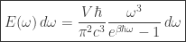
describing how much of the energy of the photon gas comes from photons of frequencies between
Planck’s law has two noteworthy limits. In the limit as 
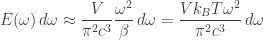
This is a form of the Rayleigh-Jeans law, which is the classical prediction for black body radiation. It’s approximately valid at low frequencies but becomes less and less accurate at higher frequencies.
Second, in the limit as 


This is a form of the Wien approximation. It’s approximately valid at high frequencies but becomes less and less accurate at low frequencies.
Both of these limits historically preceded Planck’s law itself.
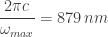
Wien’s displacement law
This form of Planck’s law is enough to tell us at what frequency the energy 
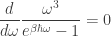
or equivalently (taking the logarithmic derivative instead)

Let 

or, with some rearrangement,

This form of the equation makes it relatively straightforward to show that there is a unique positive solution 


where 
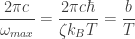
where

(the units here being meter-kelvins). This computation is typically done in a slightly different way, by first re-expressing the density of energies 


which is about 

where

This is Wien’s displacement law for wavelengths. Note that 
A wood fire has a temperature of around 


and

For comparison, the wavelengths of visible light range between about 

By contrast, the temperature of the surface of the sun is about 
and
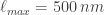
which correctly suggests that the sun is emitting lots of light all around the visible spectrum (hence appears white). In some sense this argument is backwards: probably the visible spectrum evolved to be what it is because of the wide availability of light in the particular frequencies the sun emits the most.
Finally, a more sobering calculation. Nuclear explosions reach temperatures of around 

and

These are the wavelengths of X-rays. Planck’s law doesn’t just stop at the maximum, so nuclear explosions also produce even shorter wavelength radiation, namely gamma rays. This is solely the radiation a nuclear explosion produces because it is hot, as opposed to the radiation it produces because it is nuclear, such as neutron radiation.
]]>
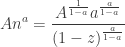
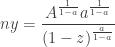
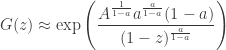
on the partition function 


The starting point is to think of a partition of 

We can make this argument into a rigorous lower bound as follows. Consider lattice paths beginning at 


whenever 


One reason this construction can’t produce a very good bound is that the partitions we get this way do not resemble the “typical” partition, which (as proven by Vershik and explained by David Speyer here) is a suitably scaled version of the curve
whereas our partitions resemble the curve 
So let’s remove the restriction that our curve resemble 


where 

and hence, when 

which (ignoring polynomial factors) is of the from 

Let

This is a major plot point in the new Ramanujan movie, where Ramanujan conjectures this result and MacMahon challenges him by agreeing to compute 
Verification
MacMahon computed

whereas the asymptotic formula gives

Ramanujan is shown getting closer than this in the movie, presumably using a more precise asymptotic.
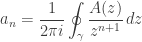
How might we conjecture such a result? In general, a very powerful method for figuring out the growth rate of a sequence 

and relate the behavior of 

The meromorphic case
The generating function strategy is easiest to carry out in the case that 
Example.The generating function for the sequence 

whose most important pole is at 


which gives, upon substituting

and hence, using the fact that
we conclude that
We ignored all of the other terms in the partial fraction decomposition to get this estimate, so there’s no reason to expect it to be particularly accurate unless 

and substituting 


If 


This is at least qualitatively the correct behavior for 

Example. A weak order is like a total order, but with ties: for example, it describes a possible outcome of a horse race. Let 

(which should be parsed as 


and hence the partial fraction decomposition of 

which gives the asymptotic

Curiously, the error in the above approximation has some funny quasi-periodic behavior corresponding to the arguments of the next most relevant poles, at 
The saddle point bound
However, understanding meromorphic functions is not enough to handle the case of partitions, where the relevant generating function is
This function is holomorphic inside the unit disk but has essential singularities at every root of unity, and to handle it we will need a more powerful method known as the saddle point method, which is beautifully explained with pictures both in Flajolet and Sedgewick and in these slides, and concisely explained in these notes by Jacques Verstraete.
The starting point is that we can recover the coefficients 

where 


From here, the name of the game is to attempt to pick 


as long as 


But later we will actually use some complex analysis to improve the saddle point bound to an estimate.
The saddle point bound gets its name from what happens when we try to optimize this bound as a function of 


and at such points the function 


and from here we can attempt to pick
We’ll often be able to write 


Example. Let 

for any 


or equivalently the lower bound

We see that the saddle point bound already gets us within a factor of
This example has a probabilistic interpretation: the saddle point bound 

which says that the probability that a Poisson random variable with rate
Example. Let 

The saddle point bound gives

for any 

with exact solution

and using 

This approximation turns out to also only be off by a factor of
Example. The Bell numbers 

(which also admits a combinatorial species description: this is the species of “sets of nonempty sets”), which as above has infinite radius of convergence. The saddle point equation is

which is approximately solved when 


Edit, 11/10/20: I don’t know how far off this is from the true asymptotics. According to Wikipedia it appears to be off by at least an exponential factor.
Example. Now let’s tackle the example of the partition function
has radius of convergence 


and it will turn out to be convenient to rearrange this a little: expanding this out gives

and exchanging the order of summation gives
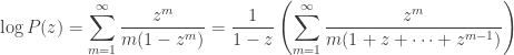
The point of writing 

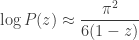
It turns out that as 

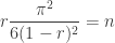
This saddle point equation reinforces the idea that 

and saddle point bound

From here we need an upper bound on 


As for the upper bound on 


from which we conclude that

and hence that

which is 
Of course, without knowing a better method that in fact gives the true answer, we have no way of independently verifying that the saddle point bounds are as close as we’ve claimed they are. We need a more powerful idea to turn these bounds into asymptotics and recover our factors of 
Hardy’s approach
In the eighth of Hardy’s twelve lectures on Ramanujan’s work, he describes a more down-to-earth way to guess that

starting from the approximation
as

for some 


based on the size of its largest term. It’s convenient to write 
so that, differentiating in 


(keeping in mind that 
and
which altogether gives (again, approximating
for 


hence 
The saddle point method
The saddle point bound, although surprisingly informative, uses very little of the information provided by the Cauchy integral formula. We ought to be able to do a lot better by picking a contour
more carefully than just by the “trivial” bound 
From here we’ll still be looking at saddle points, but more carefully, as follows. Ignoring the length factor 


If we pick
- the contour integral over a small arc (in terms of the circle method, the “major arc”) is easy to approximate (usually by a Gaussian integral), and
- the contour integral over everything else (in terms of the circle method, the “minor arc”) is small enough that it’s easy to bound.
The Gaussian integrals that often appear when integrating over the major arc are responsible for the factors of
Let’s see how this works in the case of the factorials, where 


This integral can also be thought of as coming from computing the Fourier coefficients of a suitable Fourier series. Write the integrand as 


so from here we can try to break up the integral into a “major arc” where 


and that the integral over the minor arc is negligible compared to this. This can be done, and the details are in Flajolet and Sedgewick (who take 
and hence that

which is exactly Stirling’s approximation. This computation also has a probabilistic interpretation: it says that the probability that a Poisson random variable with rate 
In general we’ll again find that, under suitable hypotheses, we can approximate the major arc integral by a Gaussian integral (using the same strategy as above) and bound the minor arc integral to show that it’s negligible. This gives the following:
Theorem (saddle point approximation): Under suitable hypotheses, if 

Directly applying this theorem to the partition function is difficult because of the difficulty of bounding what happens on the minor arc.
We will completely ignore these difficulties and pretend that only the contribution from the (saddle point near the) essential singularity at
Unfortunately there does not seem to be a really easy way to do this; Hardy’s approach uses the modular properties of the eta function, while Flajolet and Sedgewick use Mellin transforms. So at this point we’ll just quote without proof the asymptotic we need from Flajolet and Sedgewick, up to the accuracy we need, namely

Although this changes the location of the saddle point slightly, for ease of computation (and because it will lose us at worst multiplicative factors in the end) we’ll continue to work with the same approximate saddle point
as before. The saddle point approximation differs from the saddle point bound 

and second, the introduction of the denominator 

and hence

so that
which gives 


Altogether the saddle point approximation, up to a multiplicative constant, is