]]>Taihong Xiaotaihong.xiao@gmail.comA Mathematical View towards CycleGAN2017-07-05T00:00:00-07:002017-07-05T00:00:00-07:00https://prinsphield.github.io/posts/2017/07/math_view_cycleganRecently, CycleGAN is a very popular image translation method, which arouse many people’s interests. Lots of people are busy with reproducing it or designing interesting image applications by replacing the training data. However, few people have thought about its limitations, though the original paper gave some discussions about them.
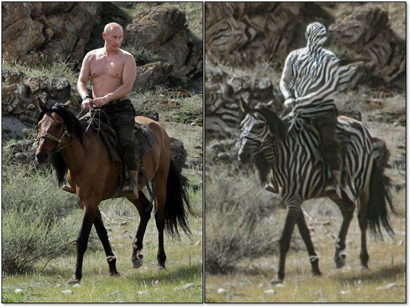
A failure case of CycleGAN was given by the author himself.
A failure case of CycleGAN.
Limitations of CycleGAN
We can actually obtain lots of information from this picture.
CycleGAN is not able to disentangle the object from the background. Putin and background are both zebraized at the same time, as shown the in the picture.
CycleGAN is suitable for global image style transfer, but weak at doing object transfiguration.
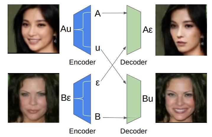
What is object transfiguration? We want to segment a certain part from an image and seamlessly implant it into another images.
For example, I want to generate a smiling face of a person by imitating the smile from another smiling face.
Smile transfiguration.
Lack of diversity in generated images, or single-modal phenomenon. For example, we use CycleGAN to do image translation between two domains. One is facial images without eyeglasses, and the other on is facial images with eyeglasses. CycleGAN can generate novel images with eyeglasses from those images without eyeglasses, but the novel eyeglasses seems always to be a black sunglasses. This phenomenon was observed by Shuchang Zhou, who was very prescient. (see our paper GeneGAN) I believe Jun-Yan Zhu, the author CycleGAN has also noticed this limitation. Otherwise, he would not publish another paper BiCycleGAN to generate multi-modal images in NIPS 2017, right after ICCV 2017 submission deadline, though the idea of BiCycleGAN is somewhat simple and the training process is very similar to IcGAN.
Weak at learning the shape of object. It is impossible if we want to use CycleGAN to generating a round object from a quadrate object.
The Reason Behind It
What cause these limitations of CycleGAN? Recall the structure of CycleGAN, there are two image domains $X$ and $Y$.
The ultimate goal of CycleGAN is to learn two maps $G$ and $F$, where $G$ maps domain $X$ to domain $Y$, and $F$ maps
domain $Y$ to domain $X$.
If $U$ is an open subset of $\mathbb{R}^n$ and $f:U\to \mathbb{R}^n$ is an injective continuous map, then $V = f(U)$ is an open
and $f$ is a homeomorphism between $U$ and $V$.
We will leave out the proof since it uses tools of algebraic topology.
This theorem tells us an important consequence:
$\mathbb{R}^n$ can not be homeomorphic to $\mathbb{R}^m$ if $m\neq n$.
Indeed, no non-empty open subset of $\mathbb{R}^n$ can be homeomorphic to any open subset of $\mathbb{R}^m$ if $m\neq n$.
Back to our discussion of CycleGAN, $G$ and $F$ are generally neural networks with auto-encoder structures, therefore continuous.
(The composition of continuous map is continuous.)
The cycle consistency guarantees that $G$ and $F$ are inverse to each other.
Therefore the domain $X$ and domain $Y$ are homeomorphic.
According to the theorem of invariance of domain, the intrinsic dimensions of $X$ and $Y$ should be the same.
This is the fundamental reason for its limitations!!!
Because the intrinsic dimensions of $X$ and $Y$ may not be the same.
For example, if we want to do image translation between domain $X$ of facial images with eyeglasses and domain $Y$ of facial images without eyeglasses. Let’s compare the intrinsic dimensions of two domains. The intrinsic dimension of domain $Y$ comes from the variety of facial images.
However, the intrinsic dimension of domain $X$ is more than that, because eyeglasses also varies, which increase the intrinsic dimensions.
In conclusion, the limitation of CycleGAN comes from the difference of intrinsic dimensions between source image domain and target image domain.
If you are interested, please read our paper GeneGAN for an alternative method.
]]>Taihong Xiaotaihong.xiao@gmail.comAn Overview on Optimization Algorithms in Deep Learning 12016-02-04T00:00:00-08:002016-02-04T00:00:00-08:00https://prinsphield.github.io/posts/2016/02/overview_opt_alg_deep_learning1Recently, I have been learning about optimization algorithms in deep learning. And it is necessary, I think, to sum them up, so I plan to write a series of articles about different kinds of these algorithms. This article will mainly talk about the basic optimization algorithms used in machine learning and deep learning.
Gradient Descent
Gradient descent is the most basic gradient-based algorithm to train a deep model. Once we get the function, let’s say $L$, that needs to optimize, especially when the function is convex, we can easily apply this method to approach the minimum of a function. This method involves updating the model parameters $\theta$ with a small step in the direction of the gradient of the objective function. For the case of supervised learning with data pairs $(x^{(i)}, y^{(i)})$, we have
where $\epsilon$ is the learning rate or the step size, that controls the size of the step the parameter takes in each iteration.
Stochastic Gradient Descent (SGD)
In spite of its impressive convergence property, batch gradient descent is rarely used in machine learning, because the cost of calculating the sum over gradient of each sample would be enormous when the number of training samples becomes large. A computationally efficient way is stochastic gradient descent in which we use the stochastic estimator of the gradient to perform its update. Based on the assumption that all samples are i.i.d, we sample one or a small suubset of $m$ training samples and compute their gradient. Then we use the gradient to update the parameter $\theta$.
When $m=1$, this algorithm is sometimes called online gradient descent. When $m>1$, the algorithm is sometimes called minibatch SGD. The algorithm is showed below.
GD or SGD, cannot escape from the occasion: if the learning rate is too big, the weights may travel to and fro across the ravine and not converge to the minimum; if the learning rate is too small, it will take a long time to converge or coonverge to local minima. Thus, we need adjust the learning rate accordingly: if the error is falliing fairly consistently but slowly, increase the learning rate; if the error keeps getting worse or oscillates wildly, then we should reduce the learning rate. Is there any algorithms that adapt the learning rate automatically?
Momentum Method
One method of speeding up training is the momentum method. This is perhaps the simplest extension to SGD that has been sucessfully used for decades. The intuition behind momentum, as the name suggests, is derived from a physical interpretation of the optimization process. Imaging a ball is rolling on a slope, the track of the ball is a combination of velocity and the instantaneous force pulling the ball downhill. And the momentum plays a role in accumulating gradient contribution.
Back to our optimization process, we want to accelerate progress along dimensions in which gradient consistently point in the same direction and to slow progress along dimensions where the sign of the gradient continues to change. This is done by keeping track of past parameter updates with an exponential decay:
where $\rho$ is a constant controlling the decay of the previous parameter updates and $\eta$ is the learning rate. The algorithm is as follows.
This gives a nice improvement over SGD when optimizing difficult cost surfaces. The issue occurred with SGD that a higher learning rate causes oscillations back and forth across the valley has been effectively solved, because the sign of gradient changes and thus the momentum term damps down these updates to slow progress across the valley. And the progress along the valley is unaffected.
Nesterov Momentum
The standard momentum method first computes the gradient at the current location and then takes a big jump in the direction of the updated accumulated gradient. Ilya Sutskever (2012 unpublished) suggested a new form of momentum that often works better. The better type of momentum is called Nesterov momentum that first make a big jump in the direction of the previous accumulated gradient, and then measure the gradient where you end up and make a correction. However, in the stochastic gradient case, Nesterov momentum does not improve the rate of convergence.
The algorithm is as follows.
]]>Taihong Xiaotaihong.xiao@gmail.comAn Overview on Optimization Algorithms in Deep Learning 22016-02-04T00:00:00-08:002016-02-04T00:00:00-08:00https://prinsphield.github.io/posts/2016/02/overview_opt_alg_deep_learning2
$$\DeclareMathOperator{\E}{E}$$
$$\DeclareMathOperator{\RMS}{RMS}$$
In the last article,
I have introduced several basic optimization algorithms. However, those algorithms rely on the hyperparameter - the learning rate $\eta$ that has a significant impact on model performance. Though the use of momentum can go some way to alleviate these issues, it does so by introducing another hyperparameter $\rho$ that may be just as difficult to set as the original learning rate. In the face of this, it’s naturally to find other way to set learning rate automatically.
AdaGrad
AdaGrad algorithm adapts the learning rates of all model parameters by scaling them inversely proportional to the accumulated sum of squared partial derivatives over all training iterations. The update rule for AdaGrad is as follows:
Here the denominator computes the $l^2$ norm of all previous gradients on a per-dimension basis and $\eta$ is a global learning rate shared by all dimensions.
The AdaGrad algorithm relies on the first order information but has some properties of second order methods and annealing. Since the dynamic rate grows with the inverse of gradient magnitudes, large gradients have smaller learning rates and small gradients have large learning rates. This nice property, as in second order methods, makes progress along each dimension even out over time. This is very useful in deep learning model, because the scale of gradients in each layer varies by several orders of magnitude. Additionally, the denominator of the scaling coefficient has the same effects as annealing, reducing the learning rate over time.
RMSprop
The RMSprop algorithm addresses the deficiency of AdaGrad by changing the gradient accumulation into an exponentially weighted moving average. In deep networks, directions in parameter space with strong partial derivatives may flatten out early, so RMSprop introduces a new hyperparameter $\rho$ that controls the length scale of the moving average to prevent that from happening.
RMSprop with Nesterov momentum algorithm is shown below.
Adam
Adam is another adaptive learning rate algorithm presented below. It can been seen as a combination of RMSprop and momentum. Adam algorithm includes bias corrections to the estimates of both the first order moment and second order moment to prevent parameters from high bias early in training.
AdaDelta
This method was derived from AdaGrad in order to improve upon the two main drawbacks of the method:
the continual decay of learning rates throughout training;
the need for a manually selected global learning rate.
Instead of accumulating the sum of squared gradients over all time, we restricted the window of past gradients that are accumulated to be some fixed size $w$ instead of size $t$ where $t$ is the current iteration as in AdaGrad. Since storing $w$ previous squared gradients is inefficient, our methods implements this accumulation as an exponentially decaying average of the squared gradients. Assume at time $t$ this running average is $\E(g^2)_t$ then we compute
\[\E(g^2)_t = \rho \E(g^2)_{t-1} +(1-\rho)g_t^2\]
Since we require the square root of this quantity in the parameter updates, this effectively becomes the RMS of previous squared gradients up to time $t$
Since the RMS of the previous gradients is already presented in the denominator in \eqref{eq-1}, we considered a measure of the $\Delta\theta$ quantity in the numerator. By computing the exponentially decaying RMS over a window of size $w$ of previous $\Delta\theta$ to give the AdaDelta method:
where the same constant $\epsilon$ is added to the numerator RMS as well to ensure progress continues to be made even if previous updates becomes small.
Extra boon: A pdf-format cheet sheet containing all these algorithms could be downloaded here for reference.
]]>Taihong Xiaotaihong.xiao@gmail.comMaximum Likelihood and Bayes Estimation2016-01-29T00:00:00-08:002016-01-29T00:00:00-08:00https://prinsphield.github.io/posts/2016/01/MSE_and_Bayes_estimation
$$\DeclareMathOperator{\E}{E}$$
$$\DeclareMathOperator{\KL}{KL}$$
$$\DeclareMathOperator{\Var}{Var}$$
$$\DeclareMathOperator{\Bias}{Bias}$$
As we know, maximum likelihood estimation (MLE) and Bayes estimation (BE) are two kinds of methods for parameter estimation in machine learning. However, they are on behalf of different view but closely interconnected with each other. In this article, I would like to talk about the differences and connections of them.
Maximum Likelihood Estimation
Consider a set of $N$ examples $\mathscr{X}=\{x^{(1)},\ldots, x^{(N)}\}$ drawn independently from the true but unknown data generating distribution $p_{data}(x)$. Let $p_{model}(x; \theta)$ be a parametric family of probability distributions over the same space indexed by $\theta$. In other words, $p_{model}(x;\theta)$ maps any $x$ to a real number estimating the true probability $p_{data}(x)$.
The maximum likelihood estimator for $\theta$ is then defined by
Since rescaling the cost function does not change the result of $\mathop{\arg\max}$, so we can divide by $N$ to obtain a formula expressed as an expectation.
One way to interprete MLE is to view what we are minimizing the dissimilarity between the experical distribution defined by training set and the model distribution, with the degree of dissimilarity between the two distributions measured by the KL divergence. The KL divergence is given by
Since the expectation of $\log \hat{p}_{data}(x)$ is a constant, we can see the optimal $\theta$ of maximum likelihood principle attempts to minimize the KL divergence.
Bayes Estimation
As discussed above, the frequentist perspective is the true parameter $\theta$ is fixed but unknown, while the MLE $\theta_{ML}$
is a random variable on account of it being a function of the data. But the bayesian perspective on statistics is quite different.
The data is intuitively observed rather than viewed randomly. They use prior probability distribution $p(\theta)$ to reflect some
knowledge they know about the distribution to some degree. Now that we have observed a set of data samples
$\mathscr{X}={x^{(1)},\ldots,x^{(N)}}$, we can recover possibility or our belief about a certain value $\theta$ by combining
the prior with the conditional distribution $p(\mathscr{X}|\theta)$ via bayes formula
Unlike what we did in MLE, Bayes estimation was effected with respect to a full distribution over $\theta$.
The quintessential idea of bayes estimation is minimizing conditional risk or expected loss function $R(\hat{\theta}|X)$, given by
where $\Theta$ is the parameter space of $\theta$. If we take the loss function to be quadratic function, i.e. $\lambda(\hat{\theta},\theta)=(\theta-\hat{\theta})^2$, then the bayes estimation of $\theta$ is
It is worth mentioning that in bayes learning, we need not to estimate $\theta$. Instead, we could give the probability distribution function of a sample $x$ directly. For example, after obsering $N$ data samples, the predicted distribution of the next example $x^{(N+1)}$, is given by
A more commonn way to estimate parameters is ccarried out using a so called maximum a posteriori (MAP) method. The MAP estimate choose the point of maximal posterior probability
As we talked above, Maximizing likelihood function is equivalent to minimizing the KL divergence between model distribution and empirical distribution. In a bayesian view of this, we can say that MLE is equivalent to minimizing empirical risk when the loss function is taken to be the logarithm loss (cross entropy loss).
The advatage brought by introducing the influence of the prior on MAP estimate is to leverage the additional information other than the unpredicted data. This additional information helps us to reduce the variance in MAP point estimate in comparison to MLE, however at the expense of increasing the bias. A good example help illustrate this idea.
Example: (Linear Regression) The problem is to find appropriate $w$ such that a mapping defined by
\[y=w^T x\]
gives the best prediction of $y$ over the entire training set $\mathscr{X}=\{x^{(1)}, \ldots,x^{(N)}\}$. Expressing the predition in a matrix form,
\[y= \mathscr{X}^T w\]
Besides, let us asssume the conditional distribution of $y$ given $w$ and $\mathscr{X}$ is Gaussian distribution parametrized by mean vector $\mathscr{X}^T w$ and variance matrix $I$.
In this case, the MLE gives an estimate
We also assume the prior of $w$ is another Gaussian distribution parametrized by mean $0$ and variance matrix $\Lambda_0=\lambda_0I$. With the prior specified, we can now determine the posterior distribution over the model parameters.
\[\hat{w}_{MAP} = (\mathscr{X}^T\mathscr{X} + \lambda_0^{-1}I)^{-1}\mathscr{X}^T y. \tag 2 \label{eq-2}\]
Compared \eqref{eq-2} with \eqref{eq-1}, we see that the MAP estimate amounts to adding a weighted term related with variance of prior distribution in the parenthesis at the basis of MLE. Also, it is easy to show that the MLE is unbiased, i.e. $\E(\hat{w}_{ML})=w$ and that it has a variance given by
\[\Bias(\hat{w}_{MAP}) = \E(\hat{w}_{MAP}) - w = -(\lambda_0\mathscr{X}^T\mathscr{X} + I)^{-1}w.\]
Therefore, we can conclude that the MAP estimate is unbiased, and as the variance of prior $\lambda_0 \to \infty$, the bias tends to $0$. And as the variance of the prior $\lambda_0 \to 0$, the bias tends to $w$. This case is exactly the ML estimate, because the variance tending to $\infty$ implies that the prior distribution is asymptotically uniform. In other words, knowing nothing about the prior distribution, we assign the same probability to every value of $w$.
It is perhaps difficult to compare \eqref{eq-3} and \eqref{eq-4}. But if we take a look at one-dimensional case, it becomes easier to see that, as long as $\lambda_0 >1$,
From the above analysis, we can see that the MAP estimate reduces the variance at the expense of increasing the bias. However, the goal is to prevent overfitting.