A Tale of Two Lambdas: A Haskeller’s Journey Into Ocaml
November 6, 2025
Jane Street, 250 Vesey St, New York, NY 10007

https://www.meetup.com/ny-haskell/events/311160463

NOTE: Please RSVP if you plan to attend. If you arrive unannounced, we’ll do our best to get you a visitor badge so you can attend, but it’s a last minute scramble for the security staff.

Schedule
6:00–6:30: Meet and Greet
6:30–8:30: Presentation
8:30–10:00: Optional Social Gathering @ a nearby bar

Speaker: Richard Eisenberg

Richard Eisenberg is a Principal Researcher at Jane Street and a leading figure in the Haskell community. His work focuses on programming language design and implementation, with major contributions to GHC, including dependent types and type system extensions. He is widely recognized for advancing the expressiveness and power of Haskell’s type system while making these ideas accessible to the broader functional programming community.

Abstract

After spending a decade focusing mostly on Haskell, I have spent the last three years looking deeply at Ocaml. This talk will capture some lessons learned about my work in the two languages and their communities — how they are similar, how they differ, and how each might usefully grow to become more like the other. I will compare Haskell’s purity against Ocaml’s support for mutation, type classes against modules as abstraction paradigms, laziness against strictness, along with some general thoughts about language philosophy. We’ll also touch on some of the challenges both languages face as open-source products, in need of both volunteers and funding. While some functional programming experience will definitely be helpful, I’ll explain syntax as we go — no Haskell or Ocaml knowledge required, as I want this talk to be accessible equally to the two communities.

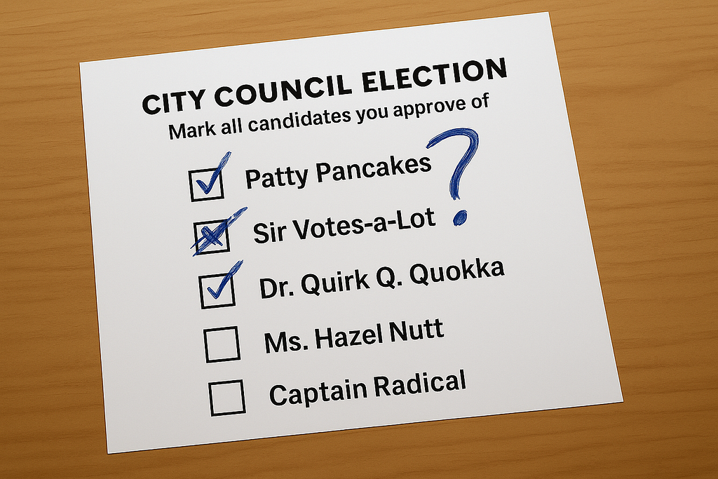
I have written previously about how approval and range voting methods are intrinsically tactical. This doesn’t mean that they are more tactical than other election systems (nearly all of which are shown to sometimes be tactical by Gibbard’s Theorem when there are three or more options). Rather, it means that tactical voting is unavoidable. Voting in such a system requires answering the question of where to set your approval threshold or how to map your preferences to a ranged voting scale. These questions don’t have more or less “honest” answers. They are always tactical choices.

But I haven’t dug deeper into what these tactics look like. Here, I’ll do the mathematical analysis to show what effective voting looks like in these systems, and make some surprising observations along the way.

Mathematical formalism for approval voting

We’ll start by assuming an approval election, so the question is where to put your threshold. At what level of approval do you switch from voting not to approve a candidate to approving them?

We’ll keep the notation minimal:

• As is standard in probability, I’ll write ℙ[X] for the probability of an event X, and 𝔼[X] for the expected value of a (numerical) random variable X.
• I will use B to refer to a random collection (multiset) of ballots, drawn from some probability distribution reflecting what we know from polling and other information sources on other voters. B will usually not include the approval vote that you’re considering casting, and to include that approval, we’ll write B ∪ {c}, where c is the candidate you contemplate approving.
• I’ll write W(·) to indicate the winner of an election with a given set of ballots. This is the candidate with the most approvals. We’ll assume some tiebreaker is in place that’s independent of individual voting decisions; for instance, candidates could be shuffled into a random order before votes are cast, in in the event of a tie for number of approvals, we’ll pick the candidate who comes first in that shuffled order.
• U(·) will be your utility function, so U(c) is the utility (i.e., happiness, satisfaction, or perceived social welfare) that you personally will get from candidate c winning the election. This doesn’t mean you have to be selfish, per se, as accomplishing some altruistic goal is still a form of utility, but we evaluate that utility from your point of view even though other voters may disagree.

With this notation established, we can clearly state, almost tautologically, when you should approve of a candidate c. You should approve of c whenever:

𝔼[U(W(B ∪ {c}))] > 𝔼[U(W(B))]

That’s just saying you should approve of c if your expected utility from the election with your approval of c is more than your utility without it.

The role of pivotal votes and exact strategy

This inequality can be made more useful by isolating the circumstances in which your vote makes a difference in the outcome. That is, W(B ∪ {c}) ≠ W(B). Non-pivotal votes contribute zero to the net expectation, and can be ignored.

In approval voting, approving a candidate can only change the outcome by making that candidate the winner. This means a pivotal vote is equivalent to both of:

• W(B ∪ {c}) = c
• W(B) ≠ c

It’s useful to have notation for this, so we’ll define V(B, c) to mean that W(B ∪ {c}) ≠ W(B), or equivalently, that W(B ∪ {c}) = c and W(B) ≠ c. To remember this notation, recall that V is the pivotal letter in the word “pivot”, and also visually resembles a pivot.

With this in mind, the expected gain in utility from approving c is:

• 𝔼[U(W(B ∪ {c}))] - 𝔼[U(W(B))]. But since the utility gain is zero except for pivotal votes, this is the same as
• ℙ[V(B, c)] · (𝔼[U(W(B ∪ {c})) | V(B, c)] - 𝔼[U(W(B)) | V(B, c)]). But since V(B, c) implies that W(B ∪ {c}) = c, so this simplifies to
• ℙ[V(B, c)] · (U(c) - 𝔼[U(W(B)) | V(B, c)])

Therefore, you ought to approve of a candidate c whenever

U(c) > 𝔼[U(W(B)) | V(B, c)]

This is much easier to interpret. You should approve of a candidate c precisely when the utility you obtain from c winning is greater than the expected utility in cases where c is right on the verge of winning (but someone else wins instead).

There are a few observations worth making about this:

• The expectation clarifies why the threshold setting part of approval voting is intrinsically tactical. It involves evaluating how likely each other candidate is to win, and using that information to compute an expectation. That means advice to vote only based on internal feelings like whether you consider a candidate acceptable is always wrong. An effective vote takes into account external information about how others are likely to vote, including polling and understanding of public opinion and mood.
• The conditional expectation, assuming V(B, c), tells us that the optimal strategy for whether to approve of some candidate c depends on the very specific situation where c is right on the verge of winning the election. If c is a frontrunner in the election, this scenario isn’t likely to be too different from the general case, and the conditional probability doesn’t change much. However, if c is a long-shot candidate from some minor party, but somehow nearly ties for a win, we’re in a strange situation indeed: perhaps a major last-minute scandal, a drastic polling error, or a fundamental misunderstanding of the public mood. Here, the conditonal expected utility of an alternate winner might be quite different from your unconditional expectation. If, say, voters prove to have an unexpected appetite for extremism, this can affect the runner-ups, as well.
• Counter-intuitively, an optimal strategy might even involve approving some candidates that you like less than some that you don’t approve! This can happen because different candidates are evaluated against different thresholds. Therefore, a single voter’s best approval ballot isn’t necessarily monotonic in their utility rankings. This adds a level of strategic complexity I hadn’t anticipated in my earlier writings on strategy in approval voting.

Approximate strategy

The strategy described above is rigorously optimal, but not at all easy to apply. Imagining the bizarre scenarios in which each candidate, no matter how minor, might tie for a win, is challenging to do well. We’re fortunate, then, that there’s a good approximation. Remember that the utility gain from approving a candidate was equal to

ℙ[V(B, c)] · (U(c) - 𝔼[U(W(B)) | V(B, c)])

In precisely the cases where V(B, c) is a bizarre assumption that’s difficult to imagine, we’re also multiplying by ℙ[V(B, c)], which is vanishingly small, so this vote is very unlikely to make a difference in the outcome. For front-runners, who are relatively much more likely to be in a tie for the win, the conditional probability changes a lot less: scenarios that end in a near-tie are not too different from the baseline expectation.

This happens because ℙ[V(B, c)] falls off quite quickly indeed as the popularity of c decreases, especially for large numbers of voters. For a national scale election (say, about 10 million voters), if c expects around 45% of approvals, then ℙ[V(B, c)] is around one in a million. That’s a small number, telling us that very large elections aren’t likely to be decided by a one-vote margin anyway. But it’s gargantuan compared to the number if c expects only 5% of approvals. Then ℙ[V(B, c)] is around one in 10^70. That’s about one in a quadrillion-vigintillion, if you want to know, and near the scale of possibly picking one atom at random from the entire universe! The probability of casting a pivotal vote drops off exponentially, and by this point it’s effectively zero.

With that in mind, we can drop the condition on the probability in the second term, giving us a new rule: Approve of a candidate c any time that:

U(c) > 𝔼[U(W(B))]

That is, approve of any candidate whose win you would like better than you expect to like the outcome of the election. In other words, imagine you have no other information on election night, and hear that this candidate has won. If this would be good news, approve of the candidate on your ballot. If it would be bad news, don’t.

• This rule is still tactical. To determine how much you expect to like the outcome of the election, you need to have beliefs about who else is likely to win, which still requires an understanding of polling and public opinion and mood.
• However, there is one threshold, derived from real polling data in realistic scenarios, and you can cast your approval ballot monotonically based on that single threshold.

This is no longer a true optimal strategy, but with enough voters, the exponential falloff in ℙ[V(B, c)] as c becomes less popular is a pretty good assurance that the incorrect votes you might cast by using this strategy instead of the optimal ones are extremely unlikely to matter. In practice, this is probably the best rule to communicate to voters in an approval election with moderate to large numbers of voters.

We can get closer with the following hypothetical: Imagine that on election night, you have no information on the results except for a headline that proclaims: Election Too Close To Call. With that as your prior, you ask of each candidate, is it good or bad news to hear now that this candidate has won. If it would be good news, then you approve of them. This still leaves one threshold, but we’re no longer making the leap that the pivotal condition for front-runners is unnecessary; we’re imagining a world in which at least some candidates, almost surely the front-runners, are tied. If this changes your decision (which it likely would only in very marginal cases), you can use this more accurate approximation.

Reducing range to approval voting

I promised to look at strategy for range voting, as well. Armed with an appreciation of approval strategy, it’s easy to extend this to an optimal range strategy, as well, for large-scale elections.

The key is to recognize that a range voting election with options 0, 1, 2, …, n is mathematically equivalent to an approval election where everyone is just allowed to vote n times. The number you mark on the range ballot can be interpreted as saying how many of your approval ballots you want to mark as approving that candidate.

Looking at it this way presents the obvious question: why would you vote differently on some ballots than others? In what situation could that possibly be the right choice?

• For small elections, say if you’re voting on places to go out and eat with your friends or coworkers, it’s possible that adding in a handful of approvals materially changes the election so that the optimal vote is different. Then it may well be optimal to cast a range ballot using some intermediate number.
• For large elections, though, you’re presented with pretty much exactly the same question each time, and you may as well give the same answer. Therefore, in large-scale elections, the optimal way to vote with a range ballot is always to rate everyone either the minimum or maximum possible score. This reduces a range election exactly to an approval election. The additional expressiveness of a range ballot is a siren call: by using it, you always vote less effectively than you would have by ignoring it and using only the two extreme choices.

Since we’re discussing political elections, which have relatively large numbers of voters, this answers the question for range elections, as well: Rate a candidate the maximum score if you like them better than you expect to like the outcome of the election. Otherwise, rate them the minimum score.

Summing it up

What we’ve learned, then, is that optimal voting in approval or range systems boils down to two nested rules.

• Exact rule (for the mathematically fearless): approve c iff U(c) > 𝔼[ U(W(B)) | your extra vote for c is pivotal ]. This Bayesian test weighs each candidate against the expected utility in the razor-thin worlds where they tie for first.
• Large-electorate shortcut (for everyone else): because those pivotal worlds become astronomically rare as the field grows, the condition shrinks to a single cutoff: approve (or give a maximum score) to every candidate whose victory you expect to enjoy more than you expected to like the result. (If you can, imagine only cases where you know the election is close.)

We’ve seen why the first rule is the gold standard; but the second captures virtually all of its benefit when millions are voting. Either way, strategy is inseparable from sincerity: you must translate beliefs about polling into a utility threshold, and then measure every candidate against it. We’ve also seen by a clear mathematical equivalence why range ballots add no real leverage in large-scale elections, instead only offering false choices that are always wrong.

The entire playbook fits on a sticky note: compute the threshold, vote all-or-nothing, and let the math do the rest.

Seeing Tom’s article reminded me of a CodeWorld feature which was implemented long ago, but I’m excited to share again in this brief note.

CodeWorld Recap

If you’re not familiar with CodeWorld, it’s a web-based programming environment I created mainly to teach mathematics and computational thinking to students in U.S. middle school, ages around 11 to 14 years old. The programming language is based on Haskell — well, it is technically Haskell, but with a lot of preprocessing and tricks aimed at smoothing out the rough edges. There’s also a pure Haskell mode, giving you the full power of the idiomatic Haskell language.

In CodeWorld, the standard library includes primitives for putting pictures on the screen. This includes:

• A few primitive pictures: circles, rectangles, and the like
• Transformations to rotate, translate, scale, clip, and and recolor an image
• Compositions to overlay and combine multiple pictures into a more complex picture.

Because the environment is functional and declarative — and this will be important — there isn’t a primitive to draw a circle. There is a primitive that represents the concept of a circle. You can include a circle in your drawing, of course, but you compose a picture by combining simpler pictures declaratively, and then draw the whole thing only at the very end.

Debugging in CodeWorld

CodeWorld’s declarative interface enables a number of really fun kinds of interactivity… what programmers might call “debugging”, but for my younger audience, I view as exploratory tools: ways they can pry open the lid of their program and explore what it’s doing.

There are a few of these that are pretty awesome. Lest I seem to be claiming the credit, the implementation for these features is due to two students in Summer of Haskell and then in Google Summer of Code: Eric Roberts, and Krystal Maughan.

• Not the point here, but there are some neat features for rewinding and replaying programs, zooming in, etc.
• There’s also an “inspect” mode, in which you not only see the final result, but the whole structure of the resulting picture (e.g., maybe it’s an overlay of three other pictures: a background, and two characters, and each of those is transformed in some way, and the base picture for the transformation is some other overlay of multiple parts…) This is possible because pictures are represented not as bitmaps, but as data structures that remember how the picture was built from its individual parts

Krystal’s recap blog post contains demonstrations of not only her own contributions, but the inspect window as well. Here’s a section showing what I’ll talk about now.

The inspect window is linked to the code editor! Hover over a structural part of the picture, and you can see which expression in your own code produced that part of the picture.

This is another application of the technique from Tom’s post. The data type representing pictures in CodeWorld stores a call stack captured at each part of the picture, so that when you inspect the picture and hover over some part, the environment knows where in your code you described that part, and it highlights the code for you, and jumps there when clicked.

While it’s the same technique, I really like this example because it’s not at all like an exception. We aren’t reporting errors or anything of the sort. Just using this nice feature of GHC that makes the connection between code and declarative data observable to help our users observe things about their own code.

I got nerd-sniped, so I’ll share my investigation.

For me, since the solution to the general problem wasn’t obvious, it made sense to specialize. Let’s say there are n players, and just to make the game finite, let’s say that instead of choosing any natural number, you choose a number from 1 to m. Choosing very large numbers is surely a bad strategy anyway, so intuitively I expect any reasonably large choice of m to give very similar results.

n = 2

Let’s start with the case where n = 2. This one turns out to be easy: you should always pick 1, daring your opponent to pick 1, as well. We can induct on m to prove this. If m = 1, then you are required to pick 1 by the rules. But if m > 1, suppose you pick m. Either your opponent also picks m and you both lose, or your opponent picks a number smaller than m and you still lose. Clearly, this is a bad strategy, and you always do at least as well choosing one of the first m - 1 options instead. This reduces the game to one where we already know the best strategy is to pick 1.

That wasn’t very interesting, so let’s try more players.

n = 3, m = 2

Suppose there are three players, each choosing either 1 or 2. It’s impossible for all three players to choose a different number! If you do manage to pick a unique number, then, you will be the only player to do so, so it will always be the least unique number simply because it’s the only one!

If you don’t think your opponents will have figured this out, you might be tempted to pick 2, in hopes that your opponents go for 1 to try to get the least number, and you’ll be the only one choosing 2. But this makes you predictable, so the other players can try to take advantage. But if one of the other players reasons the same way, you both are guaranteed to lose! What we want here is a Nash equilibrium: a strategy for all players such that no single player can do better by deviating from that strategy.

It’s not hard to see that all players should flip a coin, choosing either 1 or 2 with equal probability. There’s a 25% chance each that a player picks the unique number and wins, and there’s a 25% chance that they all choose the same number and all lose. Regrettable, but anything you do to try to avoid that outcome just makes your play more predictable so that the other players could exploit that.

It’s interesting to look at the actual computation. When computing a Nash equilibrium, we generally rely on the indifference principle: a player should always be indifferent between any choice that they make at random, since otherwise, they would take the one with the better outcome and always play that instead.

This is a bit counter-intuitive! Naively, you might think that the optimal strategy is the one that gives the best expected result, but when a Nash equilibrium involves a random choice— known as a mixed strategy — then any single player actually does equally well against other optimal players no matter which mix of those random choices they make! In this game, though, predictability is a weakness. Just as a poker player tries to avoid ‘tells’ that give away the strength of their hand, players in this number-choosing game need to be unpredictable. The reason for playing the Nash equilibrium isn’t that it gives the best expected result against optimal opponents, but rather that it can’t be exploited by an opponent.

Let’s apply this indifference principle. This game is completely symmetric — there’s no order of turns, and all players have the same choices and payoffs available — so an optimal strategy ought to be the same for any player. Then, let’s say p is the probability that any single player will choose 1. Then if you choose 1, you will win with probability (1 — p)², while if you choose 2, you’ll win with probability p². If you set these equal to each other as per the indifference principle, and solve the equation, you get p = 0.5, as we reasoned above.

n = 3, m = 3

Things get more interesting if each player can choose 1, 2, or 3. Now it’s possible for each player to choose uniquely, so it starts to matter which unique number you pick. Let’s say each player chooses 1, 2, and 3 with the probabilities p, q, and r respectively. We can analyze the probability of winning with each choice.

• If you pick 1, then you always win unless someone else also picks a 1. Your chance of winning, then, is (q + r)².
• If you pick 2, then for you to win, either both other players need to pick 1 (eliminating each other because of uniqueness and leaving you to win by default), or both other players need to pick 3, so that you’ve picked the least number. Your chance of winning is p² + r².
• If you pick 3, then you need your opponents to pick the same different number: either 1 or 2. Your chance of winning is p² + q².

Setting these equal to each other immediately shows us that since p² + q² = p² + r², we must conclude that q = r. Then p² + q² = (q + r)² = 4q², so p² = 3q² = 3r². Together with p + q + r = 1, we can conclude that p = 2√3 - 3 ≈ 0.464, while q = r = 2 - √3 ≈ 0.268.

This is our first really interesting result. Can we generalize?

n = 3, in general

The reasoning above generalizes well. If there are three players, and you pick a number k, you are betting that either the other two players will pick the same number less than k, or they will each pick numbers greater than k (regardless of whether they are the same one).

I’ll switch notation here for convenience. Let X be a random variable representing a choice by a player from the Nash equilibrium strategy. Then if you choose k, your probability of winning is P(X=1)² + … + P(X=k-1)² + P(X>k)². The indifference principle tells us that this should be equal for any choice of k. Equivalently, for any k from 1 to m - 1, the probability of winning when choosing k is the same as the probability when choosing k + 1. So:

• P(X=1)² + … + P(X=k-1)² + P(X>k)² = P(X=1)² + … + P(X=k)² + P(X>k+1)²
• Cancelling the common terms: P(X>k)² = P(X=k)² + P(X>k+1)²
• Rearranging: P(X=k) = √(P(X≥k+1)² - P(X>k+1)²)

This gives us a recursive formula that we can use (in reverse) to compute P(X=k), if only we knew P(X=m) to get started. If we just pick something arbitrary, though, it turns out that all the results are just multiples of that choice. We can then divide by the sum of them all to normalize the probabilities to sum to 1.

Here I can write some code (in Haskell):

import Probability.Distribution (Distribution, categorical, probabilities)

nashEquilibriumTo :: Integer -> Distribution Double Integer
nashEquilibriumTo m = categorical (zip allPs [1 ..])
  where
    allPs = go m 1 0 []
    go 1 pEqual pGreater ps = (/ (pEqual + pGreater)) <$> (pEqual : ps)
    go k pEqual pGreater ps =
      let pGreaterEqual = pEqual + pGreater
       in go
            (k - 1)
            (sqrt (pGreaterEqual * pGreaterEqual - pGreater * pGreater))
            pGreaterEqual
            (pEqual : ps)

main :: IO ()
main = print (probabilities (nashEquilibriumTo 100))

I’ve used a probability library from https://github.com/cdsmith/prob that I wrote with Shae Erisson during a fun hacking session a few years ago. It doesn’t help yet, but we’ll play around with some of its further features below.

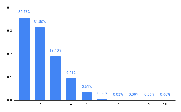
Trying a few large values for m confirms my suspicion that any reasonably large choice of m gives effectively the same result.

1 -> 0.4563109873079237
2 -> 0.24809127016999155
3 -> 0.1348844977362459
4 -> 7.333521940168612e-2
5 -> 3.987155303205954e-2
6 -> 2.1677725302500214e-2
7 -> 1.1785941067126387e-2

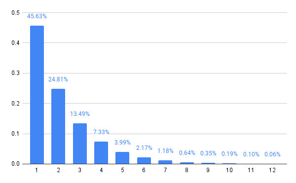
By inspection, this appears to be a geometric distribution, parameterized by the probability 0.4563109873079237. We can check that the distribution is geometric, which just means that for all k < m - 1, the ratio P(X > k) / P(X ≥ k) is the same as P(X > k + 1) / P(X ≥ k + 1). This is the defining property of a geometric distribution, and some simple algebra confirms that it holds in this case.

But what is this bizarre number? A few Google queries gets us to an answer of sorts. A 2002 Ph.D. dissertation by Joseph Myers seems to arrive at the same number in the solution to a question about graph theory, where it’s identified as the real root of the polynomial x³ - 4x² + 6x - 2. We can check that this is right for a geometric distribution. Starting with P(X=k) = √(P(X≥k+1)² -P(X>k+1)²) where k = 1, we get P(X=1) = √(P(X ≥ 2)² -P(X > 2)²). If P(X=1) = p, then P(X ≥ 2) = 1 - p, and P(X > 2) = (1 - p)², so we have p = √((1-p)² - ((1 - p)²)²), which indeed expands to p⁴ - 4p³ + 6p² - 2p = 0, so either p = 0 (which is impossible for a geometric distribution), or p³ - 4p² + 6p - 2 = 0, giving the probability seen above. (How and if this is connected to the graph theory question investigated in that dissertation, though, is certainly beyond my comprehension.)

You may wonder, in these large limiting cases, how often it turns out that no one wins, or that we see wins with each number. Answering questions like this is why I chose to use my probability library. We can first define a function to implement the game’s basic rule:

leastUnique :: (Ord a) => [a] -> Maybe a
leastUnique xs = listToMaybe [x | [x] <- group (sort xs)]

And then we can define the whole game using the strategy above for each player:

gameTo :: Integer -> Distribution Double (Maybe Integer)
gameTo m = do
  ns <- replicateM 3 (nashEquilibriumTo m)
  return (leastUnique ns)

Then we can update main to tell us the distribution of game outcomes, rather than plays:

main :: IO ()
main = print (probabilities (gameTo 100))

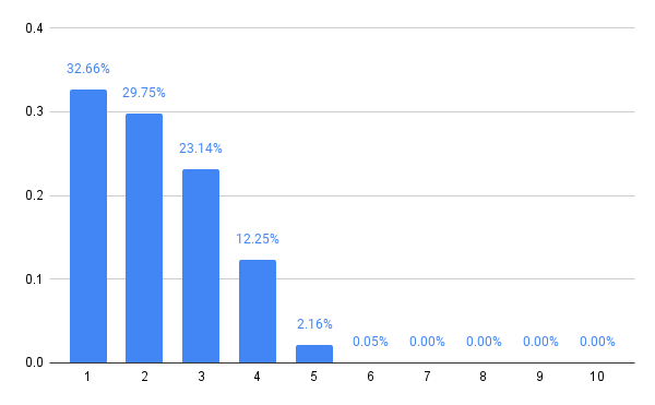
And get these probabilities:

Nothing -> 0.11320677243374572
Just 1  -> 0.40465349320873445
Just 2  -> 0.22000565820506113
Just 3  -> 0.11961465909617276
Just 4  -> 6.503317590749513e-2
Just 5  -> 3.535782320137907e-2
Just 6  -> 1.9223659987298684e-2
Just 7  -> 1.0451692718822408e-2

An 11% probability of no winner for large m is an improvement over the 25% we computed for m = 2. Once again, a least unique number greater than 7 has less than 1% probability, and the probabilities drop even more rapidly from there.

More than three players?

With an arbitrary number of players, the expressions for the probability of winning grow rather more involved, since you must consider the possibility that some other players have chosen numbers greater than yours, while others have chosen smaller numbers that are duplicated, possibly in twos or in threes.

For the four-player case, this isn’t too bad. The three winning possibilities are:

• All three other players choose the same smaller number. This has probability P(X=1)³ + … + P(X=k-1)³
• All three other players choose larger numbers, though not necessarily the same one. This has probability P(X > k)³
• Two of the three other players choose the same smaller number, and the third chooses a larger number. This has probability 3 P(X > k) (P(X=1)² + … + P(X=k-1)²)

You could possibly work out how to compute this one without too much difficulty. The algebra gets harder, though, and I dug deep enough to determine that the Nash equilibrium is no longer a geometric distribution. If you assume the Nash equilibrium is geometric, then numerically, the probability of choosing 1 that gives 1 and 2 equal rewards would need to be about 0.350788, but this choice gives too small a reward for choosing 3 or more, implying they ought to be chosen less often.

For larger n, even stating the equations turns into a nontrivial problem of accurately counting the possible ways to win. I’d certainly be interested if there’s a nice-looking result here, but I do not yet know what it is.

Numerical solutions

We can solve this numerically, though. Using the probability library mentioned above, one can easily compute, for any finite game and any strategy (as a probability distribution of moves) the expected benefit for each choice.

expectedOutcomesTo :: Int -> Int -> Distribution Double Int -> [Double]
expectedOutcomesTo n m dist =
  [ probability (== Just i) $ leastUnique . (i :) <$> replicateM (n - 1) dist
    | i <- [1 .. m]
  ]

We can then then iteratively adjust the probability of each choice slightly based on how its expected outcome compares to other expected outcomes in the distribution. It turns out to be good enough to compare with an immediate neighbor. Just so that all of our distributions remain valid, instead of working with the global probabilities P(X=k), we’ll do the computation with conditional probabilities P(X = k | X ≥ k), so that any sequence of probabilities is valid, without worrying about whether they sum to 1. Given this list of conditional probabilities, we can produce a probability distribution like this.

distFromConditionalStrategy :: [Double] -> Distribution Double Int
distFromConditionalStrategy = go 1
  where
    go i [] = pure i
    go i (q : qs) = do
      choice <- bernoulli q
      if choice then pure i else go (i + 1) qs

Then we can optimize numerically, using the difference of each choice’s win probability from its neighbor as a diff to add to the conditional probability of that choice.

refine :: Int -> Int -> [Double] -> Distribution Double Int
refine n iters strategy
  | iters == 0 = equilibrium
  | otherwise =
      let ps = expectedOutcomesTo n m equilibrium
          delta = zipWith subtract (drop 1 ps) ps
          adjs = zipWith (+) strategy delta
       in refine n (iters - 1) adjs
  where
    m = length strategy + 1
    equilibrium = distFromConditionalStrategy strategy

It works well enough to run this for 10,000 iterations at n = 4, m = 10.

main :: IO ()
main = do
  let n = 4
      m = 10
      d = refine n 10000 (replicate (m - 1) 0.3)
  print $ probabilities d
  print $ expectedOutcomesTo n m d

The resulting probability distribution is, to me, at least, quite surprising! I would have expected that more players would incentivize you to choose a higher number, since the additional players make collisions on low numbers more likely. But it seems the opposite is true. While three players at least occasionally (with 1% or more probability) should choose numbers up to 7, four players should apparently stop at 3.

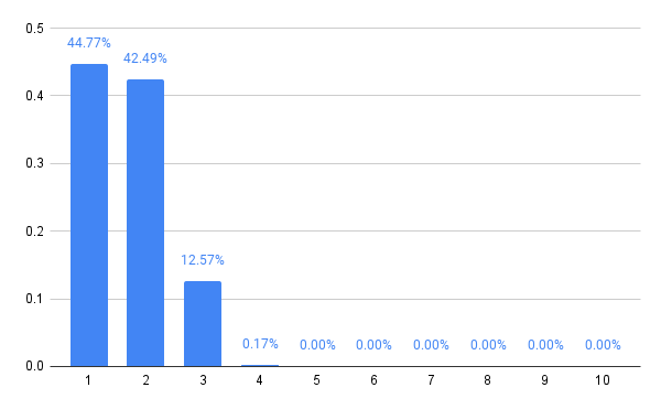
Huh. I’m not sure why this is true, but I’ve checked the computation in a few ways, and it seems to be a real phenomenon. Please leave a comment if you have a better intuition for why it ought to be so!

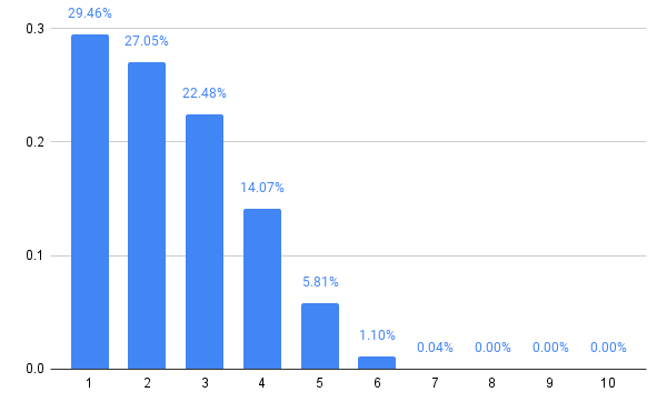
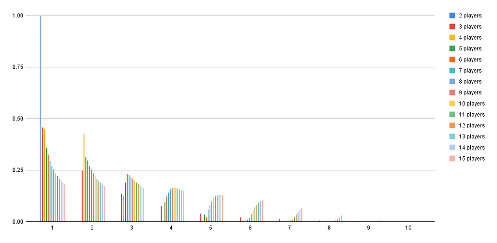
With five players, at least, we see some larger numbers again in the Nash equilibrium, lending support to the idea that there was something unusual going on with the four player case. Here’s the strategy for five players:

The six player variant retracts the distribution a little, reducing the probabilities of choosing 5 or 6, but then 7 players expands the choices a bit, and it’s starting to become a pattern that even numbers of players lend themselves to a tighter style of play, while odd numbers open up the strategy.

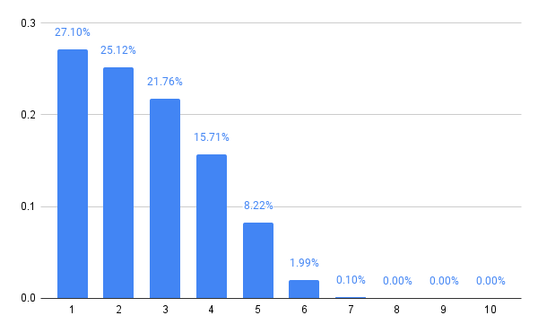
In general, it looks like this is converging to something. The computations are also getting progressively slower, so let’s stop there.

Game variants

There is plenty of room for variation in the game, which would change the analysis. If you’re looking for a variant to explore on your own, in addition to expanding the game to more players, you might try these:

• What if a tie awards each player an equal fraction of the reward for a full win, instead of nothing at all? (This actually simplifies the analysis a bit!)
• What if, instead of all wins being equal, we found the least unique number, and paid that player an amount equal to the number itself? Now there’s somewhat less of an incentive for players to choose small numbers, since a larger number gives a large payoff! This gives the problem something like a prisoner’s dilemma flavor, where players could coordinate to make more money, but leave themselves open to being undercut by someone willing to make a small profit by betraying the coordinated strategy.

What other variants might be interesting?

Addendum (Sep 26): Making it faster

As is often the case, the naive code I originally wrote can be significantly improved. In this case, the code was evaluating probabilities by enumerating all the ways players might choose numbers, and then computing the winner for each one. For large values of m and n this is a lot, and it grows exponentially.

There’s a better way. We don’t need to remember each individual choice to determine the outcome of the game in the presence of further choices. Instead, we need only determine which numbers have been chosen once, and which have been chosen more than once.

data GameState = GameState
  { dups :: Set Int,
    uniqs :: Set Int
  }
  deriving (Eq, Ord)

To add a new choice to a GameState requires checking whether it’s one of the existing unique or duplicate choices:

addToState :: Int -> GameState -> GameState
addToState n gs@(GameState dups uniqs)
  | Set.member n dups = gs
  | Set.member n uniqs = GameState (Set.insert n dups) (Set.delete n uniqs)
  | otherwise = GameState dups (Set.insert n uniqs)

We can now directly compute the distribution of GameState corresponding to a set of n players playing moves with a given distribution. The use of simplify from the probability library here is crucial: it combines all the different paths that lead to the same outcome into a single case, avoiding the exponential explosion.

stateDist :: Int -> Distribution Double Int -> Distribution Double GameState
stateDist n moves = go n (pure (GameState mempty mempty))
  where
    go 0 states = states
    go i states = go (i - 1) (simplify $ addToState <$> moves <*> states)

Now it remains to determine whether a certain move can win, given the game state resulting from the remaining moves.

win :: Int -> GameState -> Bool
win n (GameState dups uniqs) =
  not (Set.member n dups) && maybe True (> n) (Set.lookupMin uniqs)

Finally, we update the function that computes win probabilities to use this new code.

expectedOutcomesTo :: Int -> Int -> Distribution Double Int -> [Double]
expectedOutcomesTo n m dist = [probability (win i) states | i <- [1 .. m]]
  where
    states = stateDist (n - 1) dist

The result is that while I previously had to leave the code running overnight to compute the n = 8 case, I can now easily compute cases up to 15 players with enough patience. This would involve computing the winner for about a quadrillion games in the naive code, making it hopeless , but the simplification reduces that to something feasible.

It seems that once you leave behind small numbers of players where odd combinatorial things happen, the equilibrium eventually follows a smooth pattern. I suppose with enough players, the probability for every number would peak and then decline, just as we see for 4 and 5 here, as it becomes worthwhile to spread your choices even further to avoid duplicates. That’s a nice confirmation of my intuition.

Some of this I covered in earlier posts, but I’m going to construct things a little differently, so I’ll start from scratch. The Collatz conjecture is about the function f(n) defined to be n/2 if n is even, or 3n+1 if n is odd. Starting with some number (say, 7, for example) we can apply this function repeatedly to get 7, then 22, then 11, then 34, 17, 52, 26, 13, 40, 20, 10, 5, 16, 8, 4, 2, 1, and then we’ll repeat 4, 2, 1, 4, 2, 1, and so on forever. The conjecture is that no matter which positive integer you start with, you’ll always end up in that same loop of 4, 2, and 1.

For reference, it’s going to be more convenient for us to work with something called the shortcut Collatz map. The idea here is that when n is odd, we already know that 3n+1 will be even. So we can shortcut one iteration by jumping straight to (3n+1)/2, just avoiding a separate pass for the division by two that we already know will be necessary.

We tend to work in base 10 as society, but the question I asked in an article a couple weeks ago is what happens if you perform this computation in base 2 or 3, instead.

• In base 2, it’s trivial to decide if a number is even or odd, and if it’s even, to divide by two. You just look at the least significant bit, and drop it if it’s a zero!
• In base 3, it’s trivial to compute 3n+1. You just add a 1 digit to the end of the number!

We could go either way, really, and in my original article I explored both computations to see what they looked like. This time, we’ll first head deep into the base 2 side, and see where it leads us.

Collatz in Base 2

When computing the Collatz function in base 2, the computationally significant part is to multiply a base 2 number by 3. We can work this out in the standard algorithm we all learned in elementary school, working from right to left, and keeping track of a carry at each step.

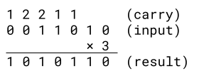
We can even enumerate the rules:

• If the next bit is a 0 and the carry is a 0, then output a 0 and carry a 0.
• If the next bit is a 1 and the carry is a 0, then output a 1 and carry a 1.
• If the next bit is a 0 and the carry is a 1, then output a 1 and carry a 0.
• If the next bit is a 1 and the carry is a 1, then output a 0 and carry a 2.
• If the next bit is a 0 and the carry is a 2, then output a 0 and carry a 1.
• If the next bit is a 1 and the carry is a 2, then output a 1 and carry a 2.

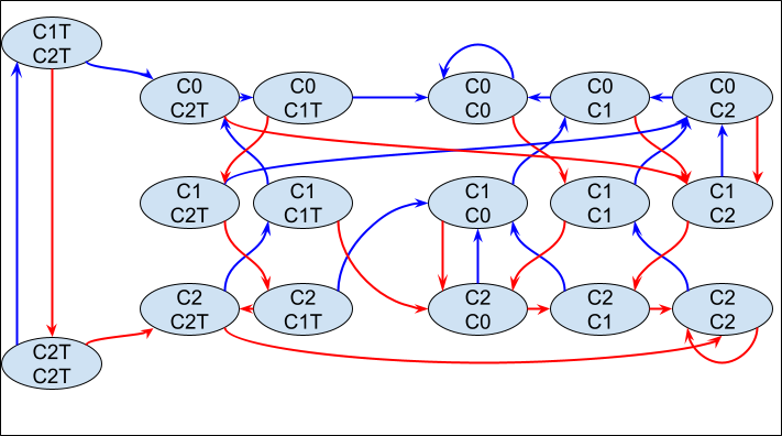
and represent this using a finite state machine with a transition diagram.

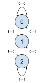
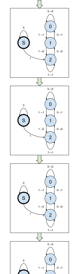
This machine isn’t too hard to understand, really. When you see a 0, move up one state; when you see a 1, move down one state. When the carry is 1 (before moving), output the opposite bit; otherwise, output the same bit. That’s all there is to it.

We will make three small modifications to this simple state machine:

• In the Collatz map, we want to compute 3n+1, That just amounts to starting with a carry of 1, rather than 0.
• Before computing 3n+1, we should divide by two until the number is odd. That amounts to adding a new “Start” state, or S for short, that ignores zeros on the right, and then acts like carry 1 when it encounters the first 1 bit. (Recall that we’re working from right to left!)
• Finally, let’s compute the shortcut map as well: as discussed above, when we compute 3n+1, it will always be even. (We will always move the start state that acts like carry 1 into carry 2, and the arrow there emits a 0 in the least significant bit.) We do not emit the zero when moving from the start state to carry 2, so the bits that come out represent (3n+1)/2.

The resulting maching looks like this.

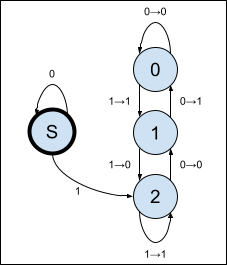
When fed the right-to-left bits of a non-zero number, this machine will compute what we might call a compressed Collatz map: dividing by 2 as long as the number remains even, and then compute (3n+1)/2 just like the shortcut Collatz map does.

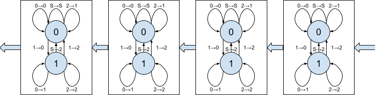
Iterating the Map

The Collatz conjecture isn’t about a single application of this map, though, but rather about the trajectory of a number when the map is applied many times in succession. To simulate this, we’ll want a whole infinite array of these machines connected end to end, so the bits that leave each one arrive at the one after. Something like this:

This is starting to get out of hand! So let’s simplify. Two things:

• Because their state transition diagrams are all the same, the only information we need about each machine is what state it’s in.
• The S state never emits any bits, and you can never get back to S once you leave it, so we know that as soon as we see an S, the entire rest of the machines, the whole infinite tail, is still sitting in the S state waiting for bits. We need not worry about these states at all.
• Once we’re done feeding in the non-zero digits of the input number, any machines in state 0 also become uninteresting. The rest of the inputs will all be zero, they will remain in state 0, and they will pass on that 0 bit of input unchanged. Again, we need not worry about these machines.

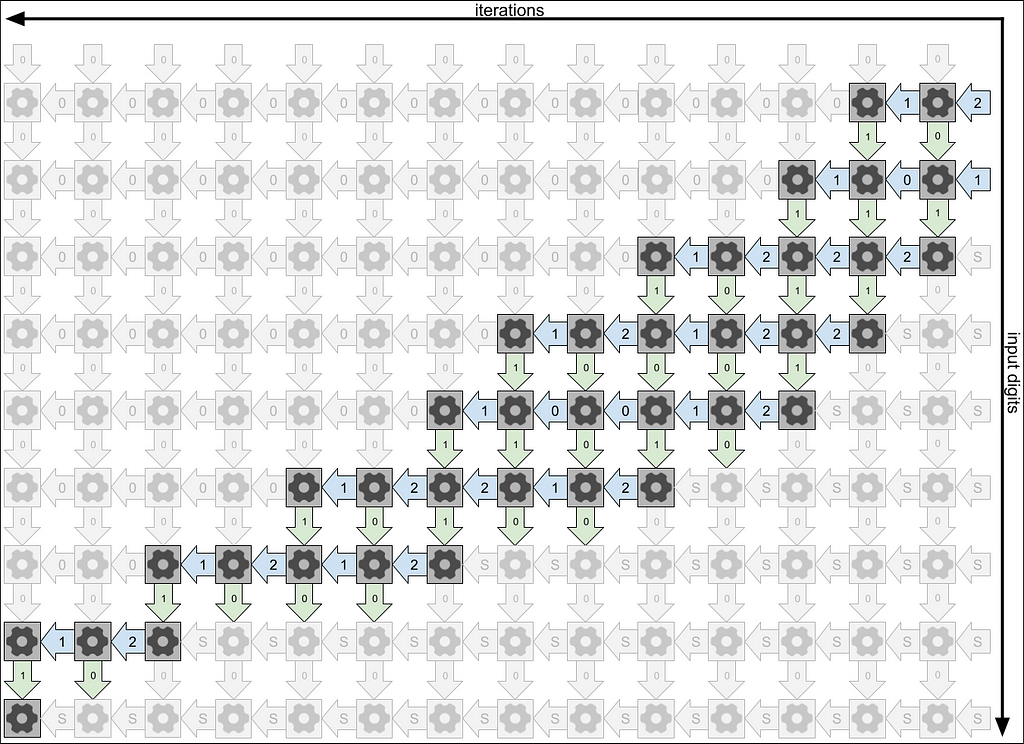
With that in mind, we can trace what happens when we feed this array of cascading machines the bits of a number. Let’s try 7, since we saw its sequence already earlier on.

The output of each machine feeds into the next machine below it, and I’ve drawn this propagation of outputs to inputs of the next machine using green arrows. We’ll draw the digits of input from right to left, matching the conventional order of writing binary numbers, so in a sense, time flows from right to left here. Each state machine remembers its state as time progresses to the left, and I’ve drawn this memory of previous states using blue arrows. Notice that to play out the full dynamics, we need to feed in quite a few of the leading zeros on the input.

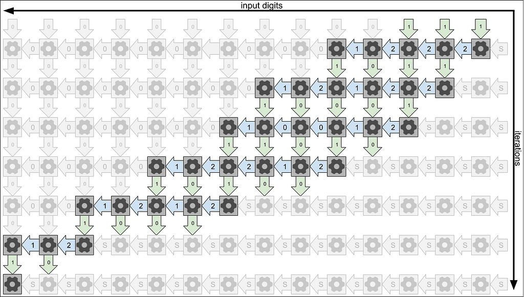
In the rows of green arrows, you can read off the outputs of each state machine in the sequence in binary:

• binary 111 = decimal 7
• binary 1011 = decimal 11
• binary 10001 = decimal 17
• binary 11010 = decimal 26
• binary 10100 = decimal 20
• binary 1000 = decimal 8
• binary 10 = decimal 2

If we were to continue, the next rows would just repeat binary 10 (decimal 2) forever. This makes sense, because the way we defined the compressed Collatz map stabilizes at 2, rather than 1.

A second thing we can read from this map is the so-called parity sequence of the shortcut Collatz map. This is just the sequence of evens and odds that occur when the map is iterated on the starting number. When a column ends by emitting a 1 bit, bumping a new machine out of the S state, that indicates that the next value of the shortcut Collatz map will be odd. When it ends in a 0 bit, then the next value will be even.

There’s quite a lot of interesting theory about the parity sequences of the shortcut Collatz map! It turns out that every possible parity sequence is generated by a unique 2-adic integer, which I defined in my previous article, so the 2-adic integers are in one-to-one correspondence with parity sequences. We can, in fact, compute the reverse direction of this one-to-one correspondence as well using state arrays like this one. Every eventually repeating parity sequence comes from a rational number, via the canonical embedding of the rationals into the 2-adic numbers. (The converse, though, that acyclic parity sequences only come from irrational 2-adic integers, is conjectured but not known!)

Because every parity sequence comes from a unique 2-adic integer, if we could show that every positive integer eventually leads to alternating even and odd numbers in its parity sequence, this would prove that the Collatz conjecture is true. Now we have a new way of looking at that question. Among the 2-adic integers, the positive integers are those that eventually have an infinite number of leading 0s. So we can ask instead, from any starting state sequence of this array of machines, when feeding zeros into the sequence forever, do we eventually (ignoring machines at the beginning that have reached the 0 state) reach only a single machine alternating through states 1, 2, 1, 2, etc.?

This isn’t an easy question, though. Certainly, feeding zeros into the array on the left will bump the state of the top-most machines down to zero. However, the bits continue to propagate through the machine, possibly pushing new machines out of their starting states and so appending them on the bottom! There is something of a race between these two processes of pruning machines on the top and adding them on the bottom, and we would need to show that the pruning wins that race.

From Base 2 to Base 3

As we investigate this race, we discover something surprising about the behavior of the state sequences when leading zeros are fed into the top machine. If you read the machine states in the blue arrows, starting at the third column from the right after all the non-zero bits of input have been fed in, we can interpret those state sequences as a ternary (base 3) number! And we get quite a familiar progression:

• ternary 222 = decimal 26
• ternary 111 = decimal 13
• ternary 202 = decimal 20
• ternary 101 = decimal 10
• ternary 12 = decimal 5
• ternary 22 = decimal 8
• ternary 11 = decimal 4
• ternary 2 = decimal 2
• ternary 1 = decimal 1

That’s the shortcut Collatz sequence again! Rather than starting at 7, we jumped three numbers ahead because it took those three steps to feed in the non-zero bits of 7, so we missed 7, 11 and 17 and went straight to 26. Then we continue according to the same dynamics.

This coincidence where state sequences can be interpreted as ternary numbers is suprising, but is it useful? It can be a revealing way to think about Collatz sequences. Here’s an example.

Numbers of the form 2ⁿ-1 have a binary representation consisting of n consecutive 1s. If we trace what happens to the state sequence, we find that each 1 we feed to this state sequence propagates all the way to the end to append another 2 to the sequence, leaving us with a state sequence consisting of n consecutive 2s. As a ternary number, that is 3ⁿ-1. If the above is correct, then, we can conclude that iterating the shortcut Collatz map n times starting with 2ⁿ-1 should yield 3ⁿ-1 as a result.

In fact, this isn’t hard to prove. We can prove the more general statement that for all i ≤ n, iterating the shortcut Collatz map i times on 2ⁿ-1 gives a result of 3ⁱ2ⁿ⁻ⁱ-1. A simple induction suffices. If i = 0, then the result is immediate. Assuming it’s true for i, and that i + 1 ≤ n, we know that 3ⁱ2ⁿ⁻ⁱ-1 is odd, so applying the shortcut Collatz map one more time yields (3(3ⁱ2ⁿ⁻ⁱ-1)+1)/2, which simplifies to establish the property for i + 1 as well, completing the induction. Now let i = n to recover the original statement.

The proof was simple, but the idea came from observing the behavior of this state machine. And this is an interesting observation: 3ⁿ-1 grows asymptotically faster than 2ⁿ-1, so it implies that there is no bound on the factor by which a number might grow in the Collatz sequence. We can always find some arbitrarily large n that grows to at least about 1.5ⁿ times its original value.

From Base 3 to Base 2

Recall that in base 3, computing 3n+1 is easy, but it’s dividing by two that becomes a non-trivial computation. Back in elementary school again, we learned about long division, an algorithm for dividing numbers digit by digit, this time left to right. To do this, we divide each digit in turn, but keep track of a remainder that propagates from digit to digit. We can also draw this as a state machine.

To extend this to the shortcut Collatz map, we need to look for a remainder when the division completes. This means that we’ll need to feed our state machine not just the ternary digits 0, 1, and 2, but an extra “Stop” signal (S for short) indicating the number is complete. Since the result may be longer than the input, it will be convenient to send an infinite sequence of these S signals, giving the machine time to output all of the digits of the result before it begins to produce S signals, as well. Upon receiving this S signal, if there is a remainder, then the input was odd, so our state machine needs to add another 2 onto the end of the sequence of ternary digits to complete the computation of (3n+1)/2 before emitting its own S signals.

Just as before, we’re interested not in a single application of this state machine, but the behavior of numbers under many different iterations, so we will again chain together an infinite number of these machines, feeding the ternary digits (or S signals) that leave each one into the next one as inputs. This time I’ll draw the ternary digits flowing from right to left.

Let’s try to simplify this picture.

• Again, all the state machines share the same transition diagram, so we need only note which state each machine is in.
• Once a machine (or the input) starts emitting S signals, it will never stop, so we need not concern outselves with these machines.
• Because the machines start in state 0 and machines in state 0 always decrease the ternary digit so no single digit can change more than two of these into non-zero states before it becomes zero itself, we’ll always encounter an infinite tail of 0 states to the left, which are similarly uninteresting.

With those simplifications in mind, we can work through the behavior of these machines starting with the input 7, which is 21 in base 3. This time, input digits (time, essentially) flows from top to bottom, while the iterations of the state machine are oriented from right to left. The green arrows represent the memory of state over time, and the blue arrows represent input and output digits.

Following the flow from right to left and reading down the blue arrows representing ternary digits, we can see the ternary values from the shortcut Collatz map computed by the state machines, read from top to bottom. We might ask a question similar to the earlier one: can we show that, starting from any state and throwing S signals at these state machines from the right, it somehow simplifies to the sequence 10 (a 0, followed by a 1 to its left), which indicates we’ve reached the cyclic orbit at 1, 2 in the shortcut Collatz sequence?

In looking at this, as you likely guessed, we find that the state sequences when read from left to right from green arrows (starting from the second row down, after all the input digits have been fed in) give the binary form of the compressed Collatz map. That’s the one that even further shortens the shortcut Collatz map by folding all the divisions by two so they happen implicitly before each odd value is processed. Starting with base 3, then, we end up back in base 2!

What’s going on? It’s easy to see that the diagram above is the same as the one from binary earlier, except for the addition of two rows at the top where we’re still feeding in the ternary digits, and some uninteresting state propagation from machines that are already emitting S signals, and swapping the interpretation of the axes. But why?

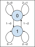
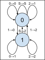
Let’s compare the state machines:

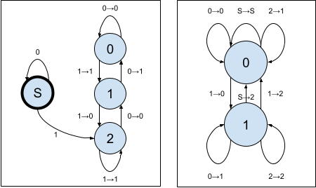
They look quite different… but this is an illusion created by a biased presentation. These diagrams emphasize the state structure, but relegate the input structure to text labels on the arrows. We can instead draw both diagrams at once in this way:

In the base 2 case, we can interpret the rows as representing bits of input, and the columns as states: three carries, and the Start state S. In the base 3 case, we can interpret the columns as inputs: three ternary digits, and the Stop signal S, and the rows as states. With either interpretation, though, the rule is the same: we are exchanging a presentation of a number from 0 through 5 as 3b + t for a presentation as 2t + b, where t takes values 0, 1, or 2, while b takes values 0 or 1, and with the same rules for the special S token on the side of the least significant digits.

So in some deep sense, computing the Collatz trajectory in base 2 or base 3 is performing the same computation. This is true even though in base 2, we’re computing the compressed Collatz map, which has fewer iterations (but more digits to compute with), while in base 3, we’re computing the shortcut Collatz map, which has more iterations (but fewer digits to compute with). Somehow these differences are all dual to each other so the same thing happens in each.

Frankly, I find that very pretty.

Brief introduction to 2-adic integers

A standard binary integer is a finite sequence of bits, either 0 or 1, with each bit having a value equal to some power of two. Because any non-negative integer can be written as a sum of powers of two, it can be written in this way.

But a finite sequence isn’t exactly right. We can always make that sequence longer, incorporating greater powers of two, by adding zeros on the left side. For this reason, if we think of a binary number as a finite sequence, we get non-unique representations: one with a 1 as the largest digit, but others that add leading zeros on the left. This is messy, so in general we tend to think of a binary integer as having infinitely many bits, but with the constraint that only finitely many of them can be non-zero. We don’t usually write the leading zeros, but that’s just a matter of notation. They are still there.

This leads to the obvious question: what happens if you remove the restriction that all but finitely many digits must be zero? The answer is the 2-adic integers. It turns out that we can write a lot of rational numbers as 2-adic integers. For example:

• Even without a negative sign, we can write -1 as …111, the 2–adic integer all of whose bits are 1. Why? Try adding one, and you’ll notice that the result is all 0s, so clearly this is the opposite of 1.
• What happens when you multiply 3 (binary 11) by the 2-adic integer …01010101011? If you work it out, you’ll get 1. So that 2-adic integer is the multiplicative inverse of 3, making it effectively 1/3.

In fact, it turns out that the 2-adic integers include all rational numbers with odd denominators! Not only that, but all of them ultimately end up with digits in a repeating pattern to the left, similar to how rational numbers in traditional decimal representations end up with digits in a repeating pattern to the right. (There are even irrational 2–adic integers that don’t repeat their digits; but they don’t correspond to the traditional irrational numbers, but rather to some completely new concept that doesn’t happen in traditional numbers!)

The Collatz map on 2-adics

The Collatz map on 2-adic integers can be defined in precisely the same way as it is on integers: even numbers are halved, while odd numbers are mapped to 3n+1. But hold on… if we can represent numbers like 1/3, what does it mean to be even or odd?

For arbitrary rationals, this would be a tricky question to answer, but in the 2–adic integers, there’s an easy answer: just look at the 1s place. If it’s 0, the number is even; if it’s 1, the number is odd. This is equivalent to saying that a rational number is even iff its numerator is even. And this notion is well-defined because we’ve already constrained the denominator to be odd.

I’m now going to redefine the Collatz step function on binary numbers from my previous post, but with one difference: I’ll assume that the numbers are odd. Because every number therefore ends with a 1, we won’t represent the 1 explicitly, but rather let it be implied. This implied 1 is expressed by the OddBits newtype.

data Bit = B0 | B1
newtype OddBits = XXX1 [Bit]
data State = C0 | C1 | C1_Trim | C2 | C2_Trim

threeNPlusOneDiv2s :: OddBits -> OddBits
threeNPlusOneDiv2s (XXX1 bits) = XXX1 (go C2_Trim bits)
  where
    go C1_Trim [] = []
    go C1_Trim (B0 : bs) = go C0 bs
    go C1_Trim (B1 : bs) = go C2_Trim bs
    go C2_Trim [] = []
    go C2_Trim (B0 : bs) = go C1_Trim bs
    go C2_Trim (B1 : bs) = go C2 bs
    go C0 [] = []
    go C0 (B0 : bs) = B0 : go C0 bs
    go C0 (B1 : bs) = B1 : go C1 bs
    go C1 [] = [B1]
    go C1 (B0 : bs) = B1 : go C0 bs
    go C1 (B1 : bs) = B0 : go C2 bs
    go C2 [] = [B0, B1]
    go C2 (B0 : bs) = B0 : go C1 bs
    go C2 (B1 : bs) = B1 : go C2 bs

This function, in a single pass, multiplies an odd number by 3, adds 1, then divides by 2 as many times as needed to make the result odd. Therefore, this is a map from the odd numbers to other odd numbers. The states represent:

1. The amount carried from the previous bit when multiplying by 3.
2. Whether the lower-order bits are all zeros, in which case we should continue to trim zeros instead of emit them.

This function still handles finite lists, but you can generally ignore those equations, since they are equivalent to extending with 0 bits to the left. And as Olaf suggests, the function extends to the 2-adic numbers by operating on infinite lists. (That is, except for one specific input: …010101, on which the function hangs non-productively. That’s because this 2-adic integer corresponds to the rational -1/3, and 3(-1/3) + 1 = 0, which can never be halved long enough to yield another odd number!)

Fixed points

The Collatz conjecture amounts to finding the orbits of the Collatz map, which fall into two categories: periodic orbits, which repeat infinitely, and divergent orbits, which grow larger indefinitely without repeating. Among positive integers, the conjecture is that the only orbit is the periodic one that ends in 4, 2, 1, 4, 2, 1, 4, 2, 1…

Since we’re skipping the even numbers, our step function has the property that f(1) = 1, making 1 a fixed point. Not all periodic orbits are fixed points, but it’s natural to ask whether there are any other fixed points of this map. Let’s explore this question!

We start by looking only at the non-terminating equations for the recursive definition. (Recall that the terminating equations are really just duplicates of these, since leading zeros are equivalent to termination.)

    go C1_Trim (B0 : bs) = go C0 bs
    go C1_Trim (B1 : bs) = go C2_Trim bs
    go C2_Trim (B0 : bs) = go C1_Trim bs
    go C2_Trim (B1 : bs) = go C2 bs
    go C0 (B0 : bs) = B0 : go C0 bs
    go C0 (B1 : bs) = B1 : go C1 bs
    go C1 (B0 : bs) = B1 : go C0 bs
    go C1 (B1 : bs) = B0 : go C2 bs
    go C2 (B0 : bs) = B0 : go C1 bs
    go C2 (B1 : bs) = B1 : go C2 bs

These observations will be relevant:

1. We start in the state C2_Trim
2. The Trim states do not emit bits to the result, only consuming them. Therefore, the output will lag behind the input by some number of bits depending on how long evaluation lingers in these Trim states.
3. Once we leave the Trim states, we can never re-enter them. Inputs and outputs will then match exactly, so the lag stays the same forever.
4. If we’re searching for inputs that evaluate in a certain way, the bits of the input are completely determined by whether we want to stay in Trim states or leave them, and then whether we want the next output to be a 0 or 1.

Because of this, when searching for a fixed point of this function, the input value is entirely determined by one choice: for how many input bits do we choose to remain in the Trim states. Once that single choice is made, the rest of the input is entirely determined by that plus the desire for the input to be a fixed point.

Let’s work some out.

Lag = 1. Here, we want to stay in the Trim states for only one bit of input. Then that bit must be a 1, since that’s what gets us out of the Trim state. From that point, we will stay in state C2, and in order to produce the 1 output bits to match the inputs, we’ll need to keep seeing 1s in the input! Then the fixed point here is XXX1 (repeat 1), which corresponds to the 2-adic integer …111.

We noted earlier that this 2–adic integer corresponds to -1. We can double-check that -1 is indeed a fixed point of the function that computes 3n+1 and then divides by 2 until the result is odd. To compute f(-1), we first compute 3(-1)+1 = -2, then divide by 2 to get -1, which is odd. So it is indeed a fixed point.

Lag = 2. Here, we want to stay in the Trim states for two bits of input. That means we expect the first bit to be 0 so that we’ll switch to state C1_Trim, and then the second bit to be 0 again to transition us to the C0 state. At this point, we’re producing output, which must match the input bits already chosen, and the input bit we need will always be a 0 so as to produce the 0 that matches the input. Then the fixed point is XXX1 (repeat 0), and keeping in mind that there’s an implied 1 on the end, this corresponds to the 2-adic integer …0001, which is just 1.

This is the standard period orbit mentioned up above: 4, 2, 1, 4, 2, 1, which is just 1s when we skip the even numbers.

Now things start to get interesting:

Lag = 3. To stay in the Trim states for exactly three bits of input, we need those bits to be 0, 1, and 1. This ends up in state C2, with the input sequence 011 left to match. The next input must therefore be 0, yielding a 0 as output, and leaving us in state C1 with 110 left to match. The next input must be 0 again, leaving us in C0 with 100 left to match. We need a 1 next, leaving us in C1 with 001 left to match. Then we need to see a 1 again to leave us in C2 with 011 left to match. That’s the same state and pending bits as we were in when we left the Trim states, so we’ve finally found a loop.

The fixed point that produces this behavior is XXX1 (cycle [0, 1, 1, 0]), and including the implied 1 on the end, this corresponds to the 2-adic integer …(0110)(0110)(0110)1. This turns out to correspond to the rational number 1/5. We can check that 3(1/5) + 1 = 8/5, and halving that three times yields 1/5 again, so this is indeed a fixed point of the map, even though it’s not an integer.

Observations about fixed points

A few observations can be made about the fixed points of this map:

1. There are an infinite number of them. Every possible choice of lag, starting with one but increasing without bound, yields a fixed point, and they all must be different since they produce different behaviors.
2. There are only a countably infinite number of them. This is the only way to produce a fixed point, so the list of fixed points we compute in this way is complete. There are no others.
3. The 2-adic fixed points are all rational. Once we leave to Trim states, there’s only a finite amount of state involved in determining what happens from here: the state of the function implementation, together with the pending input bits remaining to match, which keeps the same length. We progress through this finite number of states indefinitely, so we must eventually reach the same state twice, and from that point, the bits will follow a repeating pattern. Therefore, interpreted as a 2–adic number, they will correspond to a rational value.
4. The only integer fixed points are 1 and -1. You can see this for non-negative integers by looking at the terminating equations in the original code: the longest terminating case produces two bits at the end before ending in trailing zeros, so the lag can be no greater than 2. Similar logic applies to negative integers, which have 1s extending infinitely to the left.

In fact, if we work out what’s going on here, we find that fixpoints of this function are precisely 1 / (2ⁿ - 3) for n > 0. (In fact, n = 0 yields -1/2, which is also a fixed point as a rational, but is not a 2-adic integer so it didn’t occur in our list.)

Periodic points

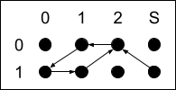
We can press further on this, and consider periodic points with period greater than one, by composing the function with itself and writing down the state machine that results. This grows more complex, as every additional iteration of the function adds a new choice about lag, yielding a larger-dimensional array of periodic points. The general form of the computation seems to remain the same, but the state diagrams grow increasingly daunting.

The diagram above gives the state transitions for the composition of two Collatz steps. The left two states are those where the first of the two steps has yet to produce a bit. The next six are states where the first is producing bits but the second is not. The final nine, then, represent the situation where both of the two composed steps is productive.

I have not labeled the outputs, but the general rule is that the trim states have no output, the non-trim states with an even number of occurrences of C1 will produce outputs that are the same as their inputs, and the states with odd occurrences of C1 produce outputs the opposite of their inputs.

Because there are now two kinds of trimming that happen, we can choose any combination of the two lags, giving a 2D array of points that repeat with period 2. The computations are similar to the above, so I’ll just give the results for lag 1, 2, and 3 in each dimension.

The diagonal elements are not new. This is expected, though, because a periodic point of period 1 is also periodic with period 2. The off-diagonal elements yield three new period-2 orbits:

• -5, -7, -5, …
• 5/7, 11/7, 5/7, …
• 7/23, 11/23, 7/23, …

Just as with fixed points, we can work out a closed form for the period two points. This time, we get (2^m + 3) / (2^(m+n) - 9). As we noticed above, this simplifies to the earlier formula for fixed points when m = n. (Hint: the denominator factors as a difference of squares.)

You might wonder if there’s a pattern here that continues to all periodic points, and indeed there is! On the Wikipedia page about the Collatz Conjecture, a formula is given for the unique rational number that generates any periodic sequence of even and odd numbers from the “shortcut” Collatz map. (The shortcut map is defined there as the map that divides by 2 once after each 3n+1 step.)

To translate this into our terms:

• m is the period, which is also the number of lag values.
• k₀ = 0, because the function defined here can only be evaluated on odd numbers.
• Each additional kᵢ is the sum of the first i lag values.
• n is the sum of all the lag values.

We can make the interesting observation that the sign of the number is determined by the denominator: if n > m log₂(3), or about 1.585 m, then the result will be positive. But n/m is also understood as the average of the lag values. So looking for positive periodic points amounts to choosing lag values with an average of greater than about 1.585. But perhaps not too much greater, if we want them to be integers, because we should not allow the denominator to grow too large. (Indeed, we saw in the fixed point case above that there was a bound on how large the lag could grow because the output needs to catch up!) Working out more precise upper bounds on lag would be an interesting step toward a search for periodic points.

The fact that this rational number is unique, left somewhat mysterious in the Wikipedia statement, comes down to the way that fixed points of these composed state machines are always determined by how long we linger in each of the trim states. The result on Wikipedia already implies that these are the only periodic points among the rationals with odd denominators. The analysis here also makes it clear that these are the only periodic points in the 2-adic integers, as well, so there are no irrational 2-adic periodic points of the Collatz map.

Of course, the trick would be to show that none of these rational values except for 1 are positive integers, and then that there are also no orbits that increase aperiodically. Actually solving the Collatz Conjecture is left as an exercise for the reader. :)

The Problem

A Collatz sequence starts with some positive integer x₀ and develops the sequence inductively as xₙ₊₁= xₙ / 2 if xₙ is even, or 3xₙ + 1 if xₙ is odd. For instance, starting with 13, we get:

• x₀ = 13
• x₁ = 3(13) + 1 = 40
• x₂ = 40 / 2 = 20
• x₃ = 20 / 2 = 10
• x₄ = 10 / 2 = 5
• x₅ = 3(5) + 1 = 16
• x₆ = 16 / 2 = 8
• x₇ = 8 / 2 = 4
• x₈ = 4 / 2 = 2
• x₉ = 2 / 2 = 1
• x₁₀ = 3(1) + 1 = 4
• x₁₁ = 4 / 2 = 2
• x₁₂ = 2 / 2 = 1

From there, it’s apparent that the sequence repeats 1, 4, 2, 1, 4, 2, … forever. That is one way for a Collatz sequence to end up. The famous question here, known as the Collatz Conjecture, is whether it’s the only way any such sequence can terminate. Not necessarily! There could be other cycles besides 1, 4, 2. Or there could be a sequence that keeps increasing forever without repeating a number. Or maybe that never happens. No one knows!

We do know a few things. First, if these things happen, they only happen with astronomically large numbers that even powerful computers haven’t been able to check by hand. We know that if even a single number is repeated, then that part of the sequence will repeat forever, since the whole tail of the sequence is determined by any single number in it. And we know that such a sequence cannot decrease forever, since Collatz sequences remain positive integers, so eventually would reach number that we know end up in the 1,4,2 loop. We also know that there are other loops in Collatz sequences that begin with negative integers, so the fact that there have been none found so far in the positive integers is at least a little surprising.

The Collatz Conjecture is famous because it’s probably one of the easiest unsolved math problem to understand the meaning of, for mathematical novices. There’s no Riemann zeta function to define. Just even and odd numbers, division by two, multiplication by three, and adding one. That doesn’t mean it’s easy to solve, though! Many mathematicians and countless novices have spent decades working on the problem, and there’s no promising road to a solution. The mathematician Erdős suggested that it’s not simply that no one has found the solution, but that mathematics is lacking even the basic tools needed to work on this problem.

Collatz and Alternate Bases

There are many, many ways to think about the Collatz conjecture, but one of them is to look at the computation in different bases. We’re not really attempting to find a more efficient way to compute Collatz sequences. If we cared about that, it would be far more efficient to use whatever representation our computing hardware is designed for! Rather, what we’re looking for here is the possibility of some kind of pattern in the computation that reveals something analytical about the problem.

Addition works essentially the same way the same regardless of base, but computations involved in multiplication and division are very dependent on the choice of base! Since the definition of the Collatz sequence two natural choices for computing Collatz sequences are base 2 (binary) and base 3 (ternary).

• In base 2, it’s trivial to decide whether a number is even or odd, and to divide by two. On the other hand, computing 3n+1 is less trivial, requiring a pass over potentially every digit in the number.
• In base 3, the opposite happens. Computing 3n+1 is now trivial. But recognizing that a number is even and dividing by two now require a pass over every digit.

Let’s jump into the details and see what happens.

Base 3 in Detail

Base 3 representations are appealing for the Collatz sequence because it’s trivial to compute 3n+1. It amounts to simply adding a 1 to the end of the representation, shifting everything else left (i.e., multiplying it by 3) to make room. If you have n = 1201 (decimal 46), for example, then 3n+1 = 12011 (demical 139).

The more difficult tasks are:

• Determining whether the number is even or odd. Unlike decimal, we cannot simply look at the last digit. Instead, a number in base 3 is even if and only if it has an even number of 1s in its representation. That’s not hard to count, but it does require looking at the entire sequence of digits.
• Dividing by two. Given a sequence of base 3 digits, we can express the division algorithm on right-to-left numbers as a state machine using the long division algorithm with remainders as states (starting with zero), using the following division table.

Let’s see how this table works with an example. Starting again with 1201 (decimal 46):

• We always start with a remainder of 0. The first digit is 1. That’s the second line of the table. The output digit is, therefore, 0, and the next remainder is 1.
• A remainder of 1 and a digit of 2 is the last line of the table. It tells us to add a 2 to the output, and proceed with a remainder of 1.
• A remainder of 1 and a digit of 0 is the fourth line. We add a 1 to the output, and proceed with a remainder of 1.
• A remainder of 1 and a digit of 1 is the fifth line. We add a 2 to the output and proceed with a remainder of 0.
• We’re now out of digits. The quotient is 0212 (decimal 23, but note that leading zero which we’ll talk about later!) and the remainder is 0.

Naively, we would have to make two passes over the current number: one to determine whether it’s even or odd, and then again, if it’s even, to divide by two. We can avoid this, though, by remembering that if a number is odd, we intend to compute 3n+1, which will always be even (because the product of two odd numbers is odd, so adding one makes it even), so we’ll then divide that by two. A little algebra reveals that (3n+1)/2 = 3(n/2 - 1/2) + 2 = 3⌊n/2⌋ + 2 if n is odd.

What this means is that we can go ahead and halve n regardless of whether it’s even or odd. At the end, we’ll know whether there’s a remainder or not, and if so, we will already be in position to append a 2 (rather than a 1 as discussed earlier) to the halved number and rejoin the original sequence. This skips one step of the Collatz sequence, but that’s okay. If our goal is only to determine whether the sequence eventually reaches 1, it doesn’t change the answer if we take this shortcut.

Appending that 2 to the end of the number changes the meaning of our state transition table a little bit. Instead of automatically quitting when we reach the end of the current number, we’ll need a chance to append another digit at the end. We’ll add rows to the table for what to do after all the digits have been seen, and be explicit about when to terminate (i.e., finish processing).

There’s one more detail we can handle as we go: as we saw earlier, dividing by two can produce a leading zero at the beginning of the result, which is unnecessary. We can arrange to never produce that leading zero at all, so we don’t need to ignore or remove it later. We just need to remember where we’re just starting and therefore don’t need to write leading zeros. In that case, the remainder is always zero, so there’s only one state to add.

We get the following state transition table.

Since there are no leading zeros in the representations, we need not concern ourselves with the case where the first digit encountered is a zero, but if you want to handle it, we can produce no output and remain in the Just Starting state, since it ought to change nothing. I’ve done so in the code below.

We can iterate this state machine on ternary numbers, and get consecutive values from the Collatz sequence, though slightly abbreviated because we combined the 3n+1 step with the following division by 2. The Collatz conjecture is now equivalent to the proposition that this iterated state machine will eventually produce only a single 1 digit.

I’ve implemented this in the Haskell programming language as follows:

import Data.Foldable (traverse_)
import System.Environment (getArgs)

data Ternary = T0 | T1 | T2 deriving (Eq, Read, Show)

step3 :: [Ternary] -> [Ternary]
step3 = si 
  where
    si (T0 : xs) = si xs
    si (T1 : xs) = s1 xs
    si (T2 : xs) = T1 : s0 xs
    si [] = []

    s0 (T0 : xs) = T0 : s0 xs
    s0 (T1 : xs) = T0 : s1 xs
    s0 (T2 : xs) = T1 : s0 xs
    s0 [] = []

    s1 (T0 : xs) = T1 : s1 xs
    s1 (T1 : xs) = T2 : s0 xs
    s1 (T2 : xs) = T2 : s1 xs
    s1 [] = [T2]

main :: IO ()
main = do
  [n] <- fmap read <$> getArgs
  traverse_ print (iterate step3 n)

And here’s a sample result:

$ cabal run exe:collatz3 ‘[T1, T2, T0, T1]’ | head -15
[T1,T2,T0,T1]
[T2,T1,T2]
[T1,T0,T2,T2]
[T1,T2,T2,T2]
[T2,T2,T2,T2]
[T1,T1,T1,T1]
[T2,T0,T2]
[T1,T0,T1]
[T1,T2]
[T2,T2]
[T1,T1]
[T2]
[T1]
[T2]
[T1]

Starting with 1201 (decimal 46), we get 212 (decimal 23), 1022 (decimal 35), 1222 (decimal 53), 2222 (decimal 80), 1111 (decimal 40), 202 (decimal 20), 101 (decimal 10), 12 (decimal 5), 22 (decimal 8), 11 (decimal 4), 2, 1, 2, 1, … As predicted, that’s the Collatz sequence, except for the omission of 3n+1 terms since their computation is merged into the following division by two.

Base 2 in Detail

So what happens in base 2 (binary)? It’s a curiously related but different story!

• Determining whether a number is even or odd is trivial: just look at the last bit and observe whether it is 0 or 1.
• Dividing an even number by two is trivial: once you observe that the last digit is a 0, simple delete it, shifting the remaining bits to the right to fill in.
• However, computing 3n+1 becomes less trivial, now requiring a pass over the entire digit sequence.

Since the hard step is multiplication, and the algorithmically natural direction to perform multiplication is from right to left, we can reverse the order in which we visit the bits, progressing from the least-significant to the most-significant. This is a change from the base 3 case, where division (the inverse of multiplication) was easier to perform in the left-to-right order.

We can start as before, by writing down a simple state transition table for a state machine that multiplies a binary number by 3. The state here is represented by the number carried to the next column.

(You might recognize this as the same table we already wrote down for halving a ternary number! The only differences are the column headers: the role of states and digits are swapped, and that we must traverse the digits in the opposite order.)

There’s one unfortunate subtlety to this table, and it has to do with leading zeros again. In principle, we think of a number in any base as having an infinite number of leading zeros on the left. In order to get correct results from this table, we need to continue consuming more digits until both the remaining digits and the current remainder are all zero. To express this, we’ll again need to convert our transition table to use explicit termination. This is so that we can stop at exactly the right point and not emit any unnecessary trailing zeros.

But what about the rest of the logic of the Collatz sequence?

• We should add one after tripling to compute 3n+1. That would also require a pass over potentially the entire number in the worst case… but we’re in luck. We can combine the two tasks just by starting from the Carry 1 state when following this state transition diagram.
• If the number is even, we should divide by two. Recall how in the ternary case, we merged some of the halving with the 3n+1 computation? This time, we can merge all the halving! Dividing even numbers by two just means dropping trailing zeros from the right side of the representation. Since we’re working right to left, it’s easy to add one more state that ignores trailing zeros at the start of the input.

We need to be a little careful here, because this version of the Collatz sequence never emits a 1, so looking for a 1 in the sequence is doomed! Instead, the numbers displayed are only the ones immediately after a 3n+1 step, so the final behavior (for all numbers computed so far, anyway) is an infinitely repeating sequence of 4s. We know from earlier that 4 is part of the 1,4,2 cycle, so seeing 4s is enough to know that the full Collatz sequence passes through 1.

We can fix this by remembering refusing to emit any of the trailing zeros. Now we’re ignoring trailing zeros, but also never producing them. The blowup in the number of states needed to keep track of whether a zero has been emitted yet is unfortunate, because we may pass through multiple states before emitting the first non-zero digit. Each of those states needs a copy that handles this new case. Here’s our final transition table.

Here’s the implementation in Haskell:

import Data.Foldable (traverse_)
import System.Environment (getArgs)

data Binary = B0 | B1 deriving (Eq, Show, Read)

step2 :: [Binary] -> [Binary]
step2 = si
  where
    si (B0 : xs) = si xs
    si (B1 : xs) = s2i xs
    si [] = [B1]

    s0 (B0 : xs) = B0 : s0 xs
    s0 (B1 : xs) = B1 : s1 xs
    s0 [] = []

    s1 (B0 : xs) = B1 : s0 xs
    s1 (B1 : xs) = B0 : s2 xs
    s1 [] = [B1]

    s1i (B0 : xs) = B1 : s0 xs
    s1i (B1 : xs) = s2i xs
    s1i [] = [B1]

    s2 (B0 : xs) = B0 : s1 xs
    s2 (B1 : xs) = B1 : s2 xs
    s2 [] = [B0, B1]

    s2i (B0 : xs) = s1i xs
    s2i (B1 : xs) = B1 : s2 xs
    s2i [] = [B1]

main :: IO ()
main = do
  [n] <- fmap read <$> getArgs
  traverse_ print (iterate step2 n)

And a result:

$ cabal run exe:collatz2 '[B1, B0, B1, B1, B0, B1]' | head -80
[B1,B0,B1,B1,B0,B1]
[B1,B0,B0,B0,B1]
[B1,B0,B1,B1]
[B1,B0,B1]
[B1]
[B1]
[B1]

We start with 101101 (45 in decimal). We triple and add one to get 136, then half to get 68, then 34, then 17, which is the next value that appears (10001 = 17 in decimal). We triple and add one to get 52, then half to get 26, then 13, which is 1101 in binary, and the third number in the list. (Remember the bits are listed from right to left!) Now triple and add one to get 40, and half until you reach 5, which is 101 in binary and the fourth number in the list. Finally, triple and add one to get 16, and half until you reach 1, which is where it stays.

Analysis

Is this a promising avenue to attack the Collatz Conjecture? Almost surely not. I’m not sure anyone knows a promising way to solve the problem. Nevertheless, we can ask what it might look like if one were to use this approach to attempt some progress on the conjecture.

One way (in fact, in some sense, the only way) to solve the Collatz Conjecture is to find some kind of quantity that:

1. Takes its minimum possible value for the number 1.
2. Always decreases from one element of a Collatz sequence to the next, except at 1.
3. Cannot decrease forever.

If such a quantity exists, then a Collatz sequence must eventually reach 1, so the Collatz Conjecture must be true — and conversely, in fact, if the Collatz Conjecture is true, then such a quantity must exist, since the number of steps to reach 1 would then be exactly such a quantity. This is equivalent to the original conjecture, which is why I commented that proving this is the only way to solve it! But this way of looking at the conjecture is interesting because it lets you define any quantity you like, as long as it has those three properties.

We know a lot of things that this quantity isn’t. It can’t be just the magnitude of the number, since that can increase with the 3n+1 rule. It also can’t be the number of digits (in any base), since that can increase sometimes, as well. Plenty of people have looked for other quantities that work. It’s useful to me to think of the quantity as a measure of the “entropy” (or rather its opposite, since it’s decreasing). It’s something you lose any time you take a step, and this tells you that eventually you will reach some minimum state, which must be the number 1.

Just guessing a quantity is unlikely to work. But if you can come to some understanding of the behavior of these computations, it’s conceivable there’s a quantity embedded in them somewhere that satisfies these conditions. If this entropy value is calculated digit by digit, you may be able to isolate how it changes in response to each of these state transition rules.

It is, at the very least, one point of view from which one might start thinking. I never claimed to have any answers! This was always just a random train of thought.

Defining the EWMA

And exponentially weighted moving average or (EWMA) is a technique often used for keeping a running estimate of some quantity as you make more observations. The idea is that each time you make a new observation, you take a weighted average of the new observation with the old average.

For a quick example, suppose you’re checking the price of gasoline every day at a nearby store.

1. On the first day it’s $3.10.
2. The second day it’s $3.20. You take the average of $3.10 and $3.20, and get $3.15 for your estimate.
3. The next day, it’s $3.30. You take the average of $3.15 and $3.30, and get $3.225 for your estimate.

This is not just the average of the three data points, which would be $3.20. Instead, the EWMA is biased in favor of more recent data. In fact, if you took these observations for a month, the first day of the month would be only about a billionth of the final result — basically ignored entirely — while the last day would amount for fully half. That’s the point: you’re looking for an estimate of the current value, so older historical data is less and less important. But you still want to smooth out the sudden jumps up and down.

In the example above, I was taking a straight average between the previous EWMA and the new data point. That leads for very short-lived data, though. More generally, there’s a parameter, normally called α, that tells you how to weight the average, giving this formula:

EWMAₙ₊₁ = xₙ₊₁ α + EWMAₙ (1-α)

In the extreme, if α = 1, you ignore the historical data and just look at the most recent value. For smaller values of α, the EWMA takes longer to adjust to the current value, but smooths out the noise in the data.

The EWMA Semigroup

Traditionally, you compute an EWMA one observation at a time, because you only make one observation at a time and keep a running average as you go. But when analyzing such a process, you may want to compute the EWMA of a large set of data in a parallel or distributed way. To do that, you’re going to look for a way to map the observations from the list into a semigroup. (See my earlier article on the relationship between monoids and list processing.)

We’ll start by looking at what the EWMA looks like on a sequence of data points x₁, x₂, …, xₙ.

• EWMA₁ = x₁
• EWMA₂ = x₁ (1-α) + x₂ α
• EWMA₃ = x₁ (1-α)² + x₂ α (1-α) + x₃ α
• EWMA₄ = x₁ (1-α)³ + x₂ α (1-α)² + x₃ α (1-α) + x₄ α

The first term of this sequence is funky and doesn’t follow the same pattern as the rest. But that’s because it was always different: since you don’t have a prior average at the first data point, you can only take the first data point itself as an expectation.

That’s a problem if we want to generate an entire semigroup from values that represent a single data point, since they would seem to all fall into this special case. We can instead treat the initial value as acting in both ways: as a prior expectation, and as an update to that expectation, giving something like this:

• EWMA₁ = x₁ (1-α) + x₁ α
• EWMA₂ = x₁ (1-α)² + x₁ α (1-α) + x₂ α
• EWMA₃ = x₁ (1-α)³ + x₁ α (1-α)² + x₂ α (1-α) + x₃ α
• EWMA₄ = x₁ (1-α)⁴ + x₁ α (1-α)³ + x₂ α (1-α)² + x₃ α (1-α) + x₄ α

The first term is the contribution of the prior expectation, but even the single observation case now has update terms, as well.

There are now two parts to the semigroup: a prior expectation, and an update rule. There’s an obvious and trivial semigroup structure to prior expectations: just take the first value and discard the later ones.

The semigroup structure on the update rules is a little more subtle. The key is to realize that the rule for updating an exponentially weighted moving average always looks a bit like the formula for EWMA₁ above: a weighted average between the prior expectation and the new target value. While single observations should use the same weight (α), composing multiple observations amounts to adjusting to a combined target value with a larger weight

It takes a little algebra to derive the new weight and target value for a composition, but it amounts to this. If:

• f₁(x) = x (1-α₁) + x₁ α₁
• f₂(x) = x (1-α₂) + x₂ α₂

Then:

• (f₁ ∘ f₂)(x) = x (1-α₃) + x₃ α₃
• α₃ = α₁ + α₂ - α₁ α₂
• x₃ = (x₁ α₁ + x₂ α₂ - x₂ α₁ α₂) / α₃

This can be defunctionalized to only store the weight and target values. In Haskell, it looks like this:

import Data.Foldable1 (Foldable1, foldMap1)
import Data.Semigroup (First (..))

data EWMAUpdate = EWMAUpdate
  { ewmaAlpha :: Double,
    ewmaTarget :: Double
  }
  deriving (Eq, Show)

instance Semigroup EWMAUpdate where
  EWMAUpdate a1 v1 <> EWMAUpdate a2 v2 =
    EWMAUpdate newAlpha newTarget
    where
      newAlpha = a1 + a2 - a1 * a2
      newTarget
        | newAlpha == 0 = 0
        | otherwise = (a1 * v1 + a2 * v2 - a1 * a2 * v2) / newAlpha

instance Monoid EWMAUpdate where
  mempty = EWMAUpdate 0 0

data EWMA = EWMA
  { ewmaPrior :: First Double,
    ewmaUpdate :: EWMAUpdate
  }
  deriving (Eq, Show)

instance Semigroup EWMA where
  EWMA p1 u1 <> EWMA p2 u2 = EWMA (p1 <> p2) (u1 <> u2)

singleEWMA :: Double -> Double -> EWMA
singleEWMA alpha x = EWMA (First x) (EWMAUpdate alpha x)

ewmaValue :: EWMA -> Double
ewmaValue (EWMA (First x) (EWMAUpdate a v)) = (1 - a) * x + a * v

ewma :: (Foldable1 t) => Double -> t Double -> Double
ewma alpha = ewmaValue . foldMap1 (singleEWMA alpha)

An EWMAUpdate is effectively a function of the form above, and its semigroup instance is reversed function composition. However, it is stored in a defunctionalized form so that the composition can be computed in advance. Then we add a few helper functions: singleEWMA to compute the EWMA for a single data point (with a given α value), ewmaValue to apply the update function to the prior and produce an estimate, and ewma to use this semigroup to compute the EWMA of any non-empty sequence.

Why?

What have we gained by looking at the problem this way?

The standard answer is that we’ve gained flexibility in how we perform the computation. In addition to computing an EWMA sequentially from left to right, we can do things like:

• Compute the EWMA in a parallel or distributed way, farming out parts of the work to different threads or machines.
• Compute an EWMA on the fly in the intermediate nodes of a balanced tree, such as one can do with Haskell’s fingertree package.

But neither of these are the reason I worked this out today. Instead, I was interested in a continuous time analogue of the EWMA. The traditional form of the EWMA is recursive, which gives you a value after each whole step of recursion, but doesn’t help much with continuous time. By working out this semigroup structure, the durations of each observation, which previously were implicit in the depth of recursion, turn into explicit weights that accumulate as different time intervals are concatenated. It’s then easy to see how you might incorporate a continuous observation with a non-unit duration, or with greater or lesser weight for some other reason.

That’s not new, of course, but it’s nice to be able to work it out simply by searching for algebraic structure.

Background and Definitions

First, some background. When an election is held, most people expect that each voter votes for some option, and the option with the most votes wins. This is called plurality voting. However, if there are more than two options, this turns out to be a terrible way to run an election! There’s a whole slew of better alternatives, but I’d like to focus on some kinds of structure that characterize them.

Let’s define some words that can describe any election, even if it looks different from the ones we’re accustomed to. In any election, some group of voters each cast a ballot, and the result of the election is determined by these ballots. More formally:

• There exists a set ℬ of possible ballots that any voter may cast. We don’t say anything about what the ballots look like. Maybe you vote for a candidate. Maybe you vote for more than one candidate. Maybe you rank the candidates. Maybe you score them. But in any case, some kind of ballot exists.
• When everyone votes, the collection of all ballots that were cast is a finite multiset of ballots, each taken from ℬ. The set of ballot collections is denoted by the Kleene star, ℬ*. By calling this a multiset, we’re assuming here that ballots are anonymous, so there can be duplicates, and we can jumble them around in any order without changing the result.

But, of course, the point of any election is to make a decision, which we call the outcome or result of the election, so:

• There exists a set ℛ of possible election results.
• There is a function r : ℬ* → ℛ giving the election result for a collection of ballots.

The main thing we care about when looking at a ballot or a collection of ballots is what effect it has on the election’s outcome. In general, there might be nominally different ways of filling out a ballot — and there usually are different collections of ballots — that have the same effect. For instance, on an approval ballot, whether you approve of everyone, approve of no one, or don’t vote at all, the effect is the same.

The mathematical way to isolate the effect of a ballot or ballots is to define an equivalence relation. We have to be careful though! A collection of ballots might give the same outcome on their own, but we also care about what effect they have when there are more ballots cast. Formally, we say:

• Two ballot collections X and Y have the same effect if, when combined with the same other ballots B, r(X ⨄ B) = r(Y ⨄ B). The symbol ⨄ just means combining two ballot collections together.
• This is an equivalence relation, so it partitions ℬ into equivalence classes. We call these equivalence classes ballot effects, and the effect of a ballot collection B is written as [B].

An example

In case that’s getting too abstract, let’s look at an example. In a three-candidate plurality election, each voter can vote for only one of the three candidates. The traditional way to count votes is to add up and report how many people voted for each candidate.

But that’s actually too much information! For example, the effect is the same whether each candidate receives 5 votes or 100 million votes, as long as they are tied. Taking the quotient by the equivalence relation above, then, discards information about vote counts that all candidates have in common, focusing only on the differences between them.

This can be conveniently visualized using a hexagonal lattice:

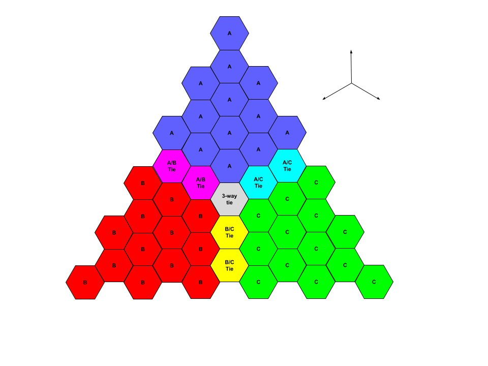
The gray space in the center represents no effect: a collection of ballots that is empty or exactly balance each other. As ballot voting for A, B, and C are added, one can move in three direction — up, down-left, and down-right — to reach the new effect.

I have only shown the effects that can be achieved with five or fewer ballots in this diagram, but the full set of effects with more ballots continues this tiling over the entire plane.

A wild monoid appears!

I’m looking for structure, and there an obvious structure to these ballot effects. We can combine two ballot effects as follows:

• Binary operation: [X] ⋅ [Y] = [X ⨄ Y]
• Identity: 1 = [∅]

Technically, one needs to verify that the binary operation is well-defined, but it’s easy to do so. It’s also associative, as combining ballot collections inherently is. Therefore, this forms a monoid E, which we will call the election monoid for this election. The election monoid describes the structure of what effects voters can have on the result of the election, and how they combine together.

Often, we may be interested not just about the effect of a collection, but also how many voters are needed to achieve that effect. In that case, we can look at subsets of the election monoid that tell us what effects can be achieved with specific numbers of ballots. This gives an ascending chain:

E₀ ⊆ E₁ ⊆ E₂ ⊆ …

This division of the election monoid into layers has a kind of compatibility with the monoid structure. Namely:

Eₘ ⋅ Eₙ ⊆ Eₘ₊ₙ

It turns out this kind of structure isn’t uncommon, and it is sometimes called filtered or graded, so that E can be described as a filtered monoid.

Looking at our three-candidate plurality election again, the nice thing about this geometric diagram is that it embeds the election monoid into a vector space, so combining effects of ballot collections amounts to just adding vectors in this space. We can also see the filtration into ballot counts.

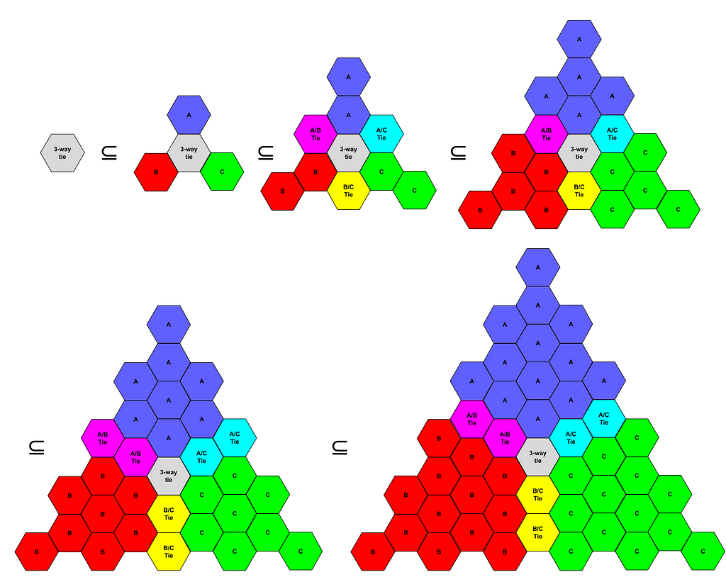
If no ballots are cast, the result is always a three-way tie. As additional ballots are cast, we can see how the set of possible outcomes grows in a triangular shape until it eventually covers the entire plane.

Application: Equal Vote Coalition’s so-called “Equality Criterion”

The Equal Vote Coalition is one of many advocacy groups promoting election reform in the United States. They primarily advocate for STAR voting, a hybrid system in which voters score candidates, then the top two candidates by average score are compared in a runoff by the number of ballots that prefer each. However, the EVC also supports other methods, including approval and a specific Condorcet method (Copeland with Borda Count as a tiebreaker, which they have branded Ranked Robin).

In support of their advocacy, they often promote something they like to call the “Equality Criterion”, even taking the unusual step of proposing it to courts as a legal standard against which to hold elections. The criterion is defined in a recent paper as follows:

The Equality Criterion states that for any given vote, there is a possible opposite vote, such that if both were cast, it would not change the outcome of an election.

In practice, if we restrict ourselves to systems with anonymous ballots as we are doing here, the main work done by this criterion is to exclude voting methods that incorporate single-choice votes among more than three candidates, including not only simple plurality voting, but also instant runoff voting (confusingly called “Ranked Choice” by some despite the wide variety of voting options that incorporate ranked choices), and hybrid methods such Smith/IRV and Tideman’s alternative method. It does not exclude score and approval voting, STAR voting, Borda count, or Condorcet methods that operate only on pairwise comparison.

Without necessarily endorsing the criterion or the claims that it relates to equality, let’s look at it through this new lens. In the notation above, this criterion says that for all x in ℬ, there exists y in ℬ such that [{x, y}] = [∅]. It’s not hard to show by a simple induction, though, that there is an equivalent statement of the property in terms of the filtered algebraic structure of vote effects.

The Algebraic “Equality Criterion”: For all n, every x in Eₙ has an inverse also in Eₙ. In other words, the election monoid is a filtered group.

Recall the three-candidate plurality election mentioned above. The effects do indeed have inverses, obtained by reflecting across the origin in the ordinary manner of a vector space. (It’s easy to check that these inverses always land back on the hexagonal grid.) However, the filtration doesn’t contain inverses for everything in each component. For example, E₂ contains the effect of putting candidate A ahead by 2 votes, but the inverse effect of putting A behind by 2 votes doesn’t occur until E₄. Therefore, a three-candidate plurality election fails the criterion.

Manufacturing “equality”

But wait! The election monoid is a group, so we were almost there. It’s only the filtration that causes the property to fail. What if we simply choose a different filtration? For the property to pass, we want to grow in a shape so that each ballot effect can be reflected across the origin and land back in the same shape. The shape that works is hexagonal rings, rather than triangles.

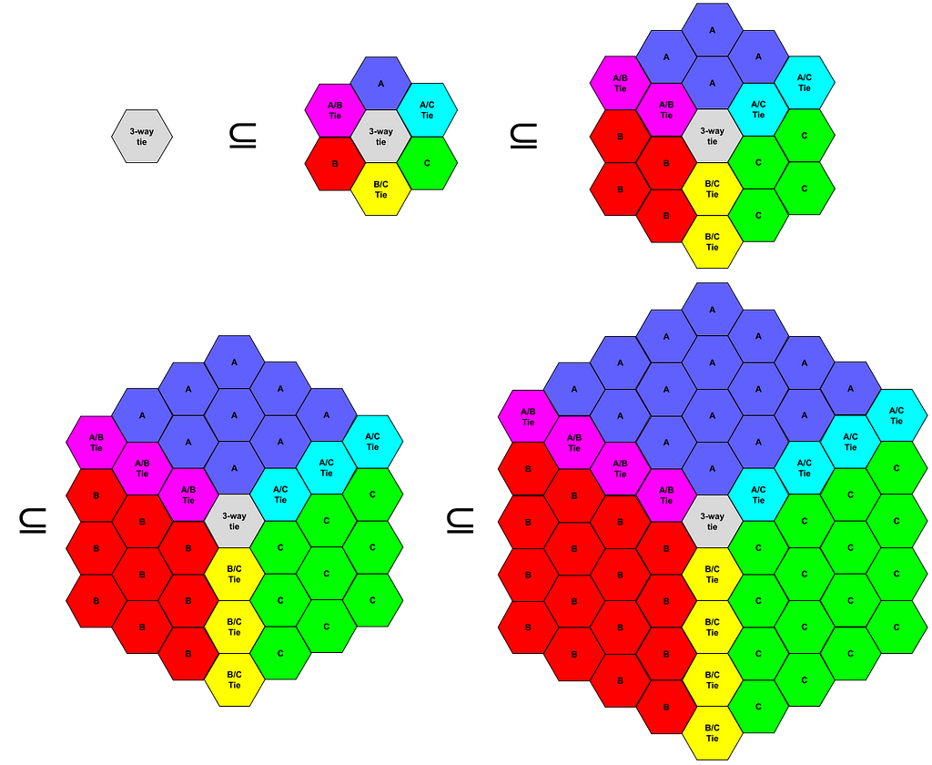
To work out what the ballots should look like to produce this filtration, take a look at the degree 1 component, representing the effects that can be achieved with a single ballot. Not only can you vote uniquely for candidates A, B, or C, you can also now vote for any two of them. (Or none, or all, but this is irrelevant since its effect is equivalent to not voting at all.) That’s an approval ballot!

Most of the common counterexamples to the criterion have this same phenomenon, where ballot effects do have inverses, but those inverses just don’t live in the same components of the filtration because it takes multiple voters to achieve them. In that case, one can follow the same process to restore the property. First, you take the degree-one component and expand it to something that includes all of its own inverses. Second, you design a ballot that can have all of those effects.

By the way, instant runoff ballot effects also have inverses. There is, indeed, a generalization of instant runoff voting that satisfies this “Equality Criterion” simply by allowing more ballots. One way to describe such a weird creature would be to have voters choose whether to use their ballot for offense, to elect their preferred candidates, or for defense, to stop the candidates they don’t want. In the latter case, the bottom-ranked candidate loses a point instead of the top-ranked candidate gaining one.

In practice, we wouldn’t consider using such a clumsy ballot in an election, but it’s as a starting point for other ideas. First, we should give a voter both effects instead just one or the other. Now we have a less crazy proposal: same ranked ballots, same instant runoff procedure, but eliminate the candidate with the worst difference between their numbers of first-place and last-place votes. We might then try some other ideas in the same spirit that use even more of the ordinal information, such as eliminating the candidate with the lowest Borda count. These may not be great ideas, but they might not be the worst systems ever proposed.

Stupid group tricks

As we saw in the last section, choosing a new filtration in this way can modify many of the election systems where this criterion fails, constructing a generalization of the system that satisfies the criterion. But this only applies if ballot effects have inverses. Sometimes, the inverses may not exist at all.

In general, if you have a commutative monoid (like the election monoid here) and would like to find inverses to make it into a group, there’s a universal method named for Alexander Grothendieck. If the election monoid is not already a group, Grothendieck’s construction can create one using pairs of ballot effects, similar to how fractions are constructed from pairs of whole numbers.

This process can be hit and miss. For instance, suppose that instead of choosing candidates, the election is about a referendum (a yes or no question), and it needs more than a mere majority to pass. This election monoid turns out to have inverses only if the threshold needed to pass the measure is a rational number. So if you want to (for whatever reason) require that the proportion of yes votes is π/4 (about 78.5%), then you get a non-invertible election monoid.

Grothendieck’s construction adds the missing inverses, but the resulting election doesn’t really retain the desired effect: instead of making “no” votes stronger than “yes” votes, it offers voters a choice of whether their vote should count more or less. Rational voters should not choose to diminish their votes, so we can remove these options. The election has now returned to a 50% threshold.

In other cases, Grothendieck’s construction is more sensible, even if the election systems it’s applied to are not! Imagine the winner is chosen using a spinner, of the style you find in children’s board games. Instead of spinning randomly, though, each player can choose to rotate it clockwise by either 1, 2, or 3 radians. Whichever candidate it lands on at the end wins.

If the votes were a rational fraction of a full turn, you could undo a vote with enough clockwise turns; for example, undoing a 1/4 turn by adding a 3/4 turn to add up to a full cycle. Here, because each vote is an irrational fraction of the full circle, there are again no inverses. Grothendieck’s construction adds inverses by allowing you to turn the spinner counter-clockwise as well.

The end of the road

There’s one case where even Grothendieck’s construction fails us: when the monoid is not cancellative. A monoid is cancellative if x⋅y = x⋅z implies that y = z. The word cancellative here refers to cancelling the x in that equation. In other words, adding the same additional ballots (x) can never make other ballots’ (y and z) have the same effect unless they already did.

A non-cancellative monoid cannot be turned into a group by adding more elements. Grothendieck’s construction will do its best, but it will forget distinctions between different ballot collections that should elect different candidates! That’s not something we can tolerate, This, then, is a fundamental limit of when we can manufacture the “Equality Criterion” for voting systems that don’t have it to begin with.

What would such an irreconcilable election system look like? Suppose you’re again voting yes or no on a referendum, but this time the rules say that we choose the result with the most votes, except that if fewer than a thousand votes are cast, the referendum automatically fails. It’s a kind of protection against sneaking through a referendum with very low turnout. Cancellativity fails here because if two ballot collections differ only in whether the participation threshold has been met, adding additional votes to each can cause them to become identical. This kind of thing happens any time you allow a fixed number of voters to irreversibly change the election.

Wrapping it up

So we constructed an algebraic approach to thinking about elections, ballots, and their effects. We then applied that to the Equal Vote Coalitions so-called “Equality Criterion”, and it revealed a connection between this criterion and a filtered group structure. By understanding that connection, we were able to see not just reword the criterion, but explore:

• The different ways in which elections might fail the criterion.
• Some universal techniques for modifying election systems to recover the criterion when it fails. One of those ended up reinventing approval voting, while another suggested some interesting IRV variants.
• Where the limits are, and when a failure of this criterion simply cannot be repaired.

To be clear, I neither endorse nor oppose this criterion, and have avoided giving my opinions on specific proposals or voting reforms. The important bit isn’t about the details of this particular criterion, but rather about what happens when we try different perspectives, look for well-understood structure, and see where that takes us.

Well, that and it was fun. Hope you enjoyed it, as well.

I ran into a problem with this specific analysis. It’s ultimately impossible to give a definitive answer for what it means to vote sincerely in an approval or score-based voting system. These voting systems force voters to make tactical choices because they do not even permit ballots that simply reflect a voter’s preferences in a straightforward way. One must make tactical decisions in order to vote at all.

I’ll explore this from two perspectives: the challenge of threshold-setting in approval voting, and the challenge of choosing a scale of voter satisfaction in score voting. Ultimately, I’ll make the claim that these are different ways of expressing the same fundamental problem.

Approval voting requires tactical threshold-setting.

You are voting in an election between three candidates: Alice, Bob, and Casey. You’re a big fan of Alice, and would love to see her elected. Bob is terrible: he kicks puppies after letting them poop on your lawn and not cleaning it up. Casey is alright; you’re not excited by them, but it wouldn’t be a disaster to see them elected. You arrive at the ballot box, and see this:

Vote for as many as you like:
[ ] Alice
[ ] Bob
[ ] Casey

What do you do? Clearly, you vote for Alice, and you don’t vote for Bob (that sassa frassin’ dirty no good puppy-kicker). But what about Casey? If you don’t vote for Casey, and then Casey comes in second just barely behind Bob, you’ll regret the decision. If you do vote for Casey, and then Casey edges out Alice for the win, you’ll also regret the decision.

This is an example of a tactical voting problem. But there’s something else going on, too. In most situations, we can think about tactical voting by comparing tactical voting to sincere voting. In this case, though, which choice is more sincere? There’s simply no good answer. You can vote for Casey to differentiate them from Bob, or you can not vote for Casey to differentiate them from Alice, but the ballot doesn’t let you explain that you prefer Alice over Casey and prefer Casey over Bob, so you are forced to make a tactical decision: which of those preferences should you express, and which should you keep to yourself?

One could argue that voters “sincerely” approve or disapprove of certain candidates, and an approval ballot can sincerely express this. However, this oversimplifies how voters perceive candidates. Preferences are relative: it’s rare to find a candidate so perfect that a voter couldn’t prefer someone else, nor so bad that a voter couldn’t imagine anyone worse. Factoring a voter’s overall level of approval —their general optimism or pessimism about politicians, for instance — into the effectiveness of their vote would be an affront to democratic principles. Everyone’s vote should count equally, regardless of their general attitude toward politics. A ballot is an expression of relative preference, not overall sentiment. In the context of approval voting, therefore, there is no objectively sincere way to decide which candidates should receive a voter’s approval.

Limited precision score voting requires tactical threshold-setting.

The same argument applies to score-based voting systems, to the extent that they offer limited precision to score candidates. We might try to fix the example above by offering an intermediate option: 1-star ratings mean you can’t stand this candidate, 2 stars means they are alright, and 3 stars means you love them. But now enter Donna, a fourth candidate who feels a bit scummy, and you’d prefer Casey to Donna, but Donna is still far better than Bob. Now you’re back in the same dilemma: you cannot merely express your preferences without making a tactical decision.

Score voting requires a tactical preference scale.

As stated above, it might seem that intrinsic tactical voting only matters when there are fewer rating choices than candidates. This isn’t the case, though. Even with essentially unlimited precision, voting systems that average voters’ scores are still inherently tactical.

Your local election is being held again, with Alice, Bob, and Casey all running for the second time. (Donna decided not to run again.) This time, the ballot reads as follows:

Rank each candidate from 1 to 100.
[ ___ ] Alice
[ ___ ] Bob
[ ___ ] Casey

You love Alice, and you’re happy to assign her a rating of 100. Bob is terrible, and clearly gets a 1. But is Casey a 25? 50? 75? The election will be decided by averaging the scores for each candidate, so if you rate Casey too high, they might edge out Alice for the win, but too low and they might be edged out by Bob.

It’s a little less obvious here that the decision of how to rate Casey is inherently tactical. Nevertheless, I’d argue that it is an inherently tactical decision, because the scale on which to rank candidates is not well-defined.

An aside about pitch

Because “satisfaction” or “happiness” are such nebulous terms, it’s easier to explain what I mean in terms that are more concrete. Let’s talk about the pitch of a musical note, which is also all about perception, but gives us a precise selection of units of measure to investigate.

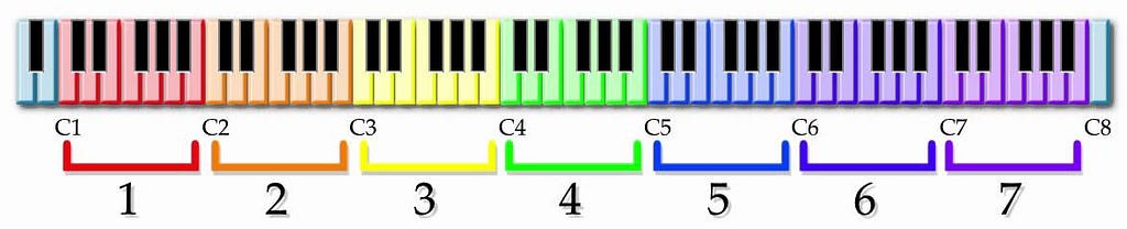
• To a musician, at least in the modern western world, pitch of musical notes is often measured in steps. Each consecutive key on a piano keyboard (including the black keys) is a half-step of difference in pitch. The distance from A2 to A4, for instance, is 24 keys, or 12 steps.
• In physics, pitch is represented by frequency, and measured in Hertz: the number of oscillations per second of the sound wave that’s produced. A2 oscillates 110 times per second, while A4 oscillates 440 times per second. That’s a difference of 330 Hertz.
• Let’s consider the note C4 (also called middle C). It’s 15 keys, or 7.5 steps, above A2. It oscillates about 262 times per second, which is 152 Hertz above A2.

Suppose a musician and a physicist are asked to rate the relative pitch of A2, C4, and A4 on a scale from 1 to 100. They both assign A2 a score of 1 because it’s the lowest pitch, and A4 a score of 100 because it’s the highest pitch. But how do they score the C4? The musician might look at the number of steps of difference: 7.5 out of 12, which is a score of about 63. The physicist might look at the frequency difference: 152 out of 330, which is a score of about 47.

Why do they reach different results? They are considering pitch on different scales with different rates of growth. These aren’t the rather boring differences we see in distance, either: whether you’re measuring in inches, centimeters, or light-years, twice as far is still twice as far. But frequency grows exponentially relative to steps, so it increases much faster in higher octaves. Conversely, steps grow logarithmically with frequency, so they increase much faster at lower frequencies and then slow down. Crucially, neither of these measurements is the right one all the time; it’s a matter of choosing a perspective and carefully defining what you’re measuring.

But what about voters and elections?

That kind of scaling issue, where there are different scales that change at different rates, is very common when we deal with perception and subjective experience, whether it’s the pitch of a sound, the brightness of a light… or, far more so, experiences of happiness or pain or satisfaction. These experiences don’t live on one definitive scale where we can compare relative distances or take averages. Rather, the scale itself is a matter of perspective, and the more subjective the experience, the harder it is to define that perspective.

So how do you rate Casey on your scored ballot? Maybe you pick a logarithmic scale, analogous to musical steps, and Casey receives a score of 63. Or maybe you pick an exponential scale, similar to frequency, and Casey receives a 47. Neither of these are fundamentally sincere or insincere ways to vote, because the ballot didn’t tell us which scale to measure on. They are simply choosing a point of view about what satisfaction means and what scale it’s best measured on.

But they do have tactical consequences: choosing the logarithmic scale that rates Casey as a 63 means using your ballot more to stop Bob from winning, while accepting that you’re doing less to help Alice beat Casey. Conversely, choosing the exponential scale that rates Casey as a 47 means using your ballot more to help Alice, and accepting that you’re doing less to help Casey beat Bob if Alice isn’t the winner.

Once again, you’re being forced to make a choice that has no sincere answer, but definitely has tactical implications. The tactics are intrinsic to the voting system.

Tactical thresholds and scales are the same thing.

These might initially seem like two very different phenomena, but I’d argue they are two manifestations of the same thing. In the first election, when you were asked to make a choice whether to approve of Casey (grouping them with Alice) or disapprove (grouping them with Bob), one way to look at this is that you were asked whether Casey is more similar to Bob or Alice in terms of how satisfied you’d be with their election.

Notice that if you adopt the logarithmic scale, where Casey scores a 63, you’re likely to consider the most sincere answer to be grouping Casey with Alice, and therefore giving them your approval. On the other hand, if you adopt the exponential scale and rate Casey a 47, you’re likely to have a tough choice, but ultimately conclude it’s more sincere to group them with Bob and not give them your approval.

In this way, the threshold-setting problem is just a consequence of the scale-setting problem. Any threshold you choose effectively defines a scale where that threshold is the midpoint between the two extremes. The precision still matters, but only in the sense that rounding error further exaggerates the difference between the scales. That is its own separate weakness, but the fact that voting is intrinsically tactical ultimately comes from the scale-setting problem in both cases.

This has consequences.

This originally came up, for me, because it made it difficult to say what it means to compare approval, range, and STAR voting systems in my simulations with sincere ballots. These voting systems do very well on many measures, such as maximizing satisfaction of voters and making decisions consistent with democratic principles like majority rule. However, when it comes to the goal of minimizing tactical voting, there’s a problem because non-tactical ballots simply do not exist. I attempted to approximate a “sincere” ballot by making these tactical choices arbitrarily, but this was rightly criticized as sub-optimal in many cases.

But outside the challenges of implementing my simulations, it has consequences for real elections, as well. An important goal in comparing election systems is to minimize the significance of tactical voting, since not all voters are equipped to vote tactically. But what does that mean when there’s no such thing as a non-tactical vote? For the same reason that I struggled to perform my analysis, voters who haven’t followed election polls and strategy closely may struggle to know how to vote at all.

With approval and score-based voting, voters are asked to cast ballots in a way that inherently involves tactical decisions, leaving no escape valve for sincere expression. This honestly can feel more like playing a complex board game than seriously assessing voter preferences. What implications might this have for voters’ decisions on whether to vote, or their confidence in the legitimacy of election results? I don’t have those answers, but they are questions worth considering.