One dimension higher, Alexander proved that every smoothly embedded 2-sphere in the 3-sphere bounds a ball on both sides. However the hypothesis of smoothness cannot be removed; in two three-page papers which appeared successively in the same volume of the Proceedings of the National Academy of Science, Alexander proved his theorem, and gave an example of a topological sphere that does not bound a ball on one side (a modified version bounds a ball on neither side). This counterexample is usually called the Alexander Horned Sphere; the `bad’ side is called a crumpled cube. For a picture of Alexander’s sphere, see this post (the `bad’ side is the outside in the figure). The horned sphere is wild; it has a Cantor set of bad points where the sphere does not have a collar; it can’t be smooth at these points.

Let’s denote the horned sphere by and the crumpled cube (i.e. the `bad’ complementary region) by . The interior of is a manifold with perfect infinitely generated fundamental group. itself is not a manifold, but it is simply connected; its `boundary’ is the topological 2-sphere . We can double to produce ; i.e. we glue two copies of together along their common boundary . It is by no means obvious how to analyze the topology of , but Bing famously proved that is . . . homeomorphic to the 3-sphere! I find this profoundly counterintuitive; on the face of it there seems to be no reason to expect is a manifold at all.

There is an obvious involution on which simply switches the two sides; it follows that there is a involution on the 3-sphere whose fixed point set is a wild 2-sphere. Bing’s proof appeared in the Annals of Mathematics; see here. This is an extremely important paper, historically speaking; it introduces for the first time Bing’s `shrinkability criterion’ for certain quotient maps to be approximable by homeomorphisms, and the ideas it introduces are a key part of the proof of the double suspension theorem and the 4-dimensional (topological) Poincare conjecture (more on this in a later post).

The paper is nine pages long, and the heart of the proof is only a couple of pages, and depends on an ingenious inductive construction. However, in Bing’s paper, this construction is indicated only by a series of four hand-drawn figures which in the first place do not obviously satisfy the property Bing claims for them, and in the second place do not obviously suggest how the sequence is to be continued. I spent several hours staring at Bing’s paper without growing any wiser, and decided it was easier to come up with my own construction than to try to puzzle out what Bing must have actually meant. So in the remainder of this blog post I will try to explain Bing’s idea, what his mysterious sequence of figures is supposed to accomplish, and say a few words about how to make this more precise and transparent.

1. The crumpled cube

First we give a precise description of the crumpled cube.

Start with the 3-ball . We will realize the crumpled cube as a subset of obtained by removing a subset defined by an infinite process.

Let denote an open solid cylinder, which we can think of technically as a 1-handle running between the centers of the disks at either end of .

We think of as a product . By the middle third of we mean the solid cylinder ; we denote this . Inside we insert two 1-handles . We attach along two disks contained in the bottom disk of , and we attach along two disks contained in the top disk of . These two 1-handles are `linked’ in as follows:

If we replace by then the union looks like this:

Denote the middle third of and by and , and replace each middle third by a pair of linked 1-handles and to obtain

And so on. Thus the crumpled cube is equal to where the index ranges over all finite strings in the alphabet . As the length of an index goes to infinity, the diameter of goes to zero, and these cylinders accumulate on a Cantor set indexed by the set of infinite binary strings. The boundary of  is a 2-sphere; this is obtained from the 2-sphere by inductively cutting out disks and gluing back the side of a cylinder and a disk at the other end, together with the limiting Cantor set

2. The crumpled cube as a quotient

The next step is to give a description of as a quotient of . Formally this is quite easy. Instead of replacing the middle third of with the 1-handles and so on, simply replace the entire solid cylinder .

In other words, we let be a pair of 1-handles attached along the boundary disks of . Note that this conflicts with our notation from the previous section. Now define and let be the intersection of this infinite family of nested solid cylinders:

The limit is a Cantor set worth of tame arcs embedded in , each running from a point on the boundary of to the corresponding point of .

By abuse of notation we can think of as a union of arcs where is an infinite binary string, obtained as obtained over all finite binary strings which are a prefix of .

To go from to we simply shrink push the boundary of into itself along the arcs , so that every arc of is pushed down to its endpoint. We start by pushing in from either end a third of the way, then push in each of from either end a third of the way, and so on; the result is evidently and it exhibits where is the equivalence relation which crushes each arc of to a point.

3. Double the picture

Now let’s double this picture.

We replace with its double . We think of the 3-sphere as together with a point at infinity, and we think of the dividing 2-sphere as the plane together with infinity. The involution acts in coordinates by taking the coordinate to its negative. The solid cylinder is doubled to a solid torus with core an unknot which we imagine as a round circle in the plane.

The solid cylinders and double to solid tori and with cores and . These are an unlink on two components; together with the core of the complement they form the three components of the Borromean rings.

In general, given any knot there is an operation which thickens the knot to a solid torus, and inserts two new knots in this solid torus, clasped as are clasped in the solid torus ; this operation is known as Bing doubling. So we can say that are obtained by Bing doubling . Inductively, we obtain by thickening which are obtained by Bing doubling , and similarly for . Bing doubling in the obvious way produces a family of nested solid tori obtained by doubling the solid cylinder , which nest down to a Cantor set of tame arcs obtained by doubling . We obtain the double of the crumpled cube as a quotient where crushes each arc of to a point.

In order not to make the pictures too complicated, we draw the shadow of each solid torus in the plane (in a rather schematic fashion). The three figures below show, successively, the torus , then inside that the shadow of , then inside that, the shadow of .

If we proceed in this way, each core has length approximately equal to , and consists roughly of two `arcs’, each of which goes half way around the core of .

4. The magic isotopy

How do we show that is homeomorphic to the 3-sphere? Bing’s idea is the following one. The arrangement of the thickened links is such that the diameter of each component in the 3-sphere is pretty big, and we must perform a quotient in the limit (which collapses the components of to points) to get . Suppose we could find a sequence of isotopies of the 3-sphere and a sequence of numbers with the following properties:

• each is supported in
• if we define then each component of with has diameter

If we could find such , then the sequence of homeomorphisms would converge to a map taking to a Cantor set in such a way that is a homeomorphism. In particular, it would descend (after taking quotients) to a homeomorphism from to .

Each isotopy, roughly speaking, `slides’ the components of with around inside the with ;  if this is done judiciously, the components can be individually moved so that their diameters are smaller than in the original configuration, and in the limit, the diameters go to zero.

As an example, we indicate how to slide inside so it only goes `a quarter’ of the way around the core of :

5. Some notation

Let’s restrict the rules of the game. We use the notation to denote the union of all with ; i.e. the union of solid tori at `depth’ . We idealize each component of as a slightly thickened circle; by abuse of notation we use the same notation to refer to the component and its core circle, assuming it is clear from context which is meant at any given time. Each of the two components of inside is idealized as a circle that starts at some point of , goes exactly half way around it, then turns around, and retraces its path to the start where it closes up. The other component starts at the same point of , but heads out in the opposite direction. Because itself is zigzagging back and forth inside its own thickened tubes, the actual image of each circle of for large jitters like crazy, and though all curves have the same length, it is conceivable that their diameters can eventually get small.

We need a bit of notation to get started.   can be thought of as a single solid unknot in in which all the successive are nested. Let’s agree that we only really need to give the angular coordinate of the core of each component of projected onto the core of (i.e. we only really care how much it `winds around the original circle’). As measured in terms of this angular coordinate, each component of each has the same length, which we normalize to . I will describe each projection by a cyclic word in the alphabet , as follows: if has length then each letter describes a segment of length which winds positively or negatively around the core of according to whether the letter is or . Thus (trivially) is given by the string , since it just winds positively once around itself.

This notation is ambiguous; it defines the image under radial projection relatively but not absolutely; it is well-defined up to the choice of a starting point. But this notation does let us compute the total angular length of the projection to the core of , which will be a good proxy for diameter. So, for example, a component associated to the word has projection angular length .

Now, suppose we have a component of some , encoded by a cyclic word , and suppose are the components of inside . We think of the letters of as segments of the loop . To build the cores of the we break into two segments each of half the length; write . Then has the same projection as and similarly for where the asterisk means the same segment with opposite orientation. We restrict ourselves to two possibilities:

• the endpoint of is at the endpoint of some segment corresponding to a letter of ; or
• the endpoint of is in the middle of some segment corresponding to a letter of .

In the first case we have a decomposition of parallel to as where are words of length . If is a word in the alphabet let be the word obtained by interchanging with and reversing the order of letters. Thus for example . With this notation, the cyclic words associated to the are and . We call the operation of replacing with the pair a split.

In the second case we must first subdivide; this means replacing by a new string by the substitution ; i.e. each letter is doubled successively. Note that by our convention and define the same radial projection (up to translation). Then as above we decompose and form and .

6. An inductive lemma

OK, we are nearly done. The initial torus  corresponds to the string consisting of a single letter . We subdivide to form and then decompose to form each with angular projection of length . We subdivide again to form and decompose to form each with angular projection of length . So far so good. But now after subdivision we have cyclic conjugates of and no matter how we split this into we will get words with some or string.

The `best’ strings are those of the form with total angular projection . Say a string is cubeless if it has no or . If is cubeless, so are the strings obtained by any split.
In a cubeless string, the only `bad’ subwords are (disjoint) substrings of the form or ; we call these runs. Our goal is to produce strings with as few runs as follows. The only strings with no runs at all are ; we call these tight.

We imagine a binary rooted tree of cyclic strings, whose node is , and such that the two children of each are obtained either from a split of or a split of . We will never double a string before splitting unless it is tight; every other string will be successively split (without doubling) until all its descendants are tight.

It is clear that Bing’s claim is proved if we can show that there is an infinite tree of this form which is a union of finite trees so that every leaf of is the cyclic string .

To prove the existence of such a tree inductively, we start at a vertex with the label and generate the part of that lies below it. That this can be done follows immediately from a lemma:

Lemma: Let be a cubeless string of even length. Then either for some , or there is a split so that each of the terms in the split have fewer runs than .

Proof:Just choose any subdivision into strings of half the length so that each of the has fewer than half of the runs of (i.e. at least one run of must be split in half by the subdivision) That this can be done follows e.g. from the intermediate value theorem. QED

One often-lamented weakness of this otherwise excellent book is that Milnor does not really give much insight into the geometric “meaning” of the characteristic classes; for example, Stiefel-Whitney classes are introduced axiomatically, and then “constructed” by appealing to the axiomatic properties of Steenrod squares, applied to the Thom class. This makes it hard to get a geometric “feel” for these classes, especially in the important case of bundles over a manifold. So I thought it would be useful to give a “geometric” description of Stiefel-Whitney classes in this context (described via Poincaré duality as cycles in the manifold), which is at the same time elementary enough to give a feel, and at the same time is transparently related to the “geometric” definition of Steenrod squares, so that one can see how the two definitions compare.

Milnor’s treatment of Stiefel-Whitney classes is axiomatic. If is an bundle over a base space , the Stiefel-Whitney classes for are the unique classes which satisfy

1. , and for ;
2. the are natural; i.e. if and is an bundle over , then if denotes the pullback bundle over (i.e. the bundle whose fiber over each is equal to the fiber of over ) then for each ;
3. the satisfy the Whitney Product Formula:  for bundles and over the same space , where and where the product in taken in the ring ; and
4. if is the twisted bundle over the circle then is nontrivial.

(For convenience, I’m going to suppress coefficients throughout the sequel.)

Uniqueness of classes satisfying these properties is established by a dimension count, after one shows that any natural characteristic class must be obtained by pulling back cohomology from a classifying map to a Grassmannian. Then Milnor shows existence via Thom’s formula involving Steenrod squares.

Explicitly, if denotes the total space of an bundle , and if denotes the complement of the zero section, there is a unique Thom class which restricts to the generator of for each fiber , and the Stiefel-Whitney classes are the unique classes in satisfying

where is projection to the base, and is the th Steenrod operation.

Well yes, exactly; clear enough if you are Thom or Milnor, but mysterious to the rest of us.

First of all, what are these Steenrod squares? They arise in a subtle way from the systematic failure of the commutativity of cup product on cohomology (with coefficients) to be represented by a commutative (and associative) product at the cochain level. Another way to say this is that they arise from the failure of cohomology classes to be represented by unique maps to classifying spaces, but rather to be represented only by unique homotopy classes of maps.

Let me explain. Let be a space and let be a class. This class is represented by a unique homotopy class of map . The external cross product class is likewise represented by a unique homotopy class of map

by pulling back a tautological class .

If acts by switching the two factors, the maps and both pull back to the same class, so they are homotopic. So there is a map which gives a homotopy from to . Likewise, we can define where switches the two factors, which gives a homotopy from to , and we can glue and together to give a map which factors through the action which switches the factors of , and acts as the antipodal map on .

But by obstruction theory, the map fills in (canonically) to a map

and we can glue and together to give

And so on by induction. In the end we obtain

which factors through the action which switches the factors of and acts as the antipodal map on . Let’s restrict to the diagonal and quotient out by to get a map

There is a ring isomorphism where has degree , and we can express the pullback of the class canonically as a polynomial in with coefficients in . This entire construction depended on the original class , so the coefficients we obtain are functions of , and these are exactly the Steenrod squares. I.e.:

for canonical classes .

This is a hell of a procedure to go through to get Stiefel-Whitney classes . So let me now explain how to “simulate” this construction geometrically to give a natural construction of Stiefel-Whitney cycles, at least in the case of a vector bundle over a manifold.

Let’s let be a closed manifold of dimension and let be a (smooth) bundle over with total space . The total space is a (noncompact) smooth manifold of dimension . We identify with a submanifold of by taking it to be the zero section, and note that this inclusion is a homotopy equivalence. Thus . It’s not hard to see that is isomorphic to the compactly supported cohomology of , so that there is a Poincaré duality isomorphism between and , and under this isomorphism, the Thom class is seen to be dual to the class represented by the zero section itself. Thus, cupping with is dual to intersection with . The Thom isomorphism is the composition with Poincaré duality in to identify with with Poincaré duality in to identify

What is ? It is Poincaré dual to a submanifold of which is Poincaré dual to the class . But the top Steenrod square is just (as can be seen from the construction above) so this is dual to the self-intersection where is obtained by perturbing so the two copies are in general position. Geometrically, we can take a generic section and let .

Okay, this identification is well-known: the top class is the obstruction to the existence of a nonzero section. Now what? We take our hint from the construction of Steenrod squares, and proceed as follows.

Since the section takes values pointwise in vector spaces, it makes sense to define the antipodal section by for each . The sections and are not equal, but at least they have the property that and are equal (ignoring signs, since we’re working over ). Now, of course any two sections of are homotopic, so we can choose a generic path of sections from to so that intersects in general position. Then define

Now, is a manifold with boundary, so we should expect this boundary to contribute a boundary to . But by construction, the two contributions to the boundary from the two points of are both equal to ; so the boundary “glues up” and we get a closed manifold, representing a homology class in  Poincaré dual to .

And now proceed by induction. The two sections and glue up to give a circle of sections which can be filled in to a disk of sections and . And so on. Each intersection is a cycle because the boundary terms all glue up by the symmetry of the construction.

Notice once we get to that by general position and symmetry each maps over the point , so that which is Poincaré dual to .

Personally I find that this construction bears a nice “family resemblance” to one of the standard constructions of Steenrod squares, and removes some of the mystery from Thom’s theorem.

One nice application of this geometric interpretation of Stiefel-Whitney cycles is that it gives an elementary proof of a theorem of Halperin-Toledo (originally conjectured by Stiefel), that if is a smooth, triangulated manifold, then the th Stiefel-Whitney class of the tangent bundle is Poincaré dual to the union of simplices in the first barycentric subdivision of the triangulation. For this reduces to Hopf’s observation that the Euler characteristic is equal mod 2 to the number of simplices (summed over all dimensions). To see this, build (in the usual way) a section of the tangent bundle over each simplex singular exactly at the vertices of the first barycentric subdivision. Then build inductively families of homotopies between these sections and their negatives in an obvious way so that they agree on the boundaries. Directly one sees that is exactly the union of the -simplices in the first barycentric subdivision.

Update 2/18/2016: Rob Kirby emailed me to point out the following nice “homework exercise”. Consider the real 1-dimensional bundle over the circle whose total space is a Mobius band. We can choose a section which is transverse to the zero section at exactly one point. Now, if we choose a (metric) connection on the bundle, then it makes sense to talk about “translating” a section by parallel transporting it around some path in the base. As we translate around the path which winds once around the base circle, it takes exactly to the section , so this is a perfectly legitimate choice of homotopy . Under this homotopy, the zero section itself zips once around the circle, and sweeps out the fundamental class; said another way, is dual to a point (the zero of the original section ) and is dual to the entire circle (the “path” of zeros of the homotopy of sections from to ).

Another Update 2/18/2016: It is natural to wonder whether there is an analog of this construction for Chern classes, at least for complex vector bundles over closed smooth oriented manifolds . It seems that there is, and it is probably worth spelling out.

If is a (smooth) bundle over with total space , then we can also think of it as a real oriented bundle (with the same total space). The image of a generic section is an oriented submanifold of the oriented total space , so we can orient the intersection and think of it as an integral homology class dual to the top Chern class . In fact, this is also the Euler class of the underlying oriented real bundle.

But now there is a natural action on the total space, coming from the natural multiplication of a vector in a complex vector space by the scalar for . So the section determines a circle’s worth of sections which can be filled in with a disk’s worth of sections . We can define and observe that the “boundary” of this manifold is just the zeros of . But the action is trivial on the set of zeros of any section, so this is in turn just equal to . In other words, the image of the boundary has codimension 2, and therefore represents a well-defined homology class dual to .

At the next stage we get by multiplying by the action. But the restriction of this action to is just rotation (since that’s how we defined on the boundary) so it factors through where the equivalence relation on quotients out the curves on this torus to points. But now observe and we actually have which can be filled in generically to , and is a cycle (as before) dual to . And so on.

Question: What is the analog in this context of the Steenrod squares? It seems they should be replaced by cohomology operations in integral cohomology, defined now not for arbitrary spaces but for spaces with actions; i.e. (presumably) they are operations on -equivariant cohomology groups. Probably such operations, and their relation to Chern classes, are classical and well known, but not by me. Can any readers fill me in?

This quarter I’m teaching an introductory graduate class on Kleinian groups. It’s something I could teach standing on my head, and during a couple of the classes I half suspected that I was. But every time I teach something, no matter how “elementary” or “familiar”, I find that I get something new out of it. This time around I have been thinking about the Schläfli formula for the variation of volume in a smooth family of hyperbolic polyhedra, and the way in which it relates to some other well-known and important volume formulae relating to hyperbolic manifolds and geometry, especially in 3 dimensions. It turns out that there are some elegant and easy ways to derive many otherwise quite complicated statements directly from Schläfli; probably this is well known to experts, but it wasn’t to me, and I think it might make an interesting blog post.

0. Volumes.

The subject of volumes is one where mathematics makes contact with daily life in many different ways. For instance, taking a shower today, I was confronted with this:

No doubt other readers with lush, voluminous hair like mine have had a similar experience.

In two dimensions volume is area. For a hyperbolic polyhedron there is a beautiful relation between the area of and the angles at the vertices. This relation (due to Gauss) is cleanest to state when is a triangle, with angles , , . For an “ordinary” triangle, the angles should all be strictly positive numbers of course. But in hyperbolic space it makes sense to consider triangles with some (or all) vertices at infinity — such vertices are called ideal, and a triangle with ideal vertices is called semi-ideal (if there are also some ordinary vertices) or ideal (if all three vertices are ideal). The group of isometries of hyperbolic space acts transitively on the set of distinct triples of points at infinity, leading to the remarkable conclusion that all ideal triangles are isometric. In particular, they all have the same area, which turns out to be .

The following diagram shows how to decompose an ideal triangle into four smaller triangles — one with angles , and the other three semi-ideal with a single non-ideal vertex with angles , and respectively.

A semi-ideal triangle with one regular vertex can be moved by an isometry so that the regular vertex is at the origin (in the unit disk model); thus one sees that such triangles are determined up to isometry by the angle at the regular vertex. Let’s use the notation for the area of such a semi-ideal triangle with regular angle . The decomposition above gives the formula

So to determine we just need to understand the function .

The next diagram shows how to decompose two semi-ideal triangles with angles and into a semi-ideal triangle with angle , and an ideal triangle.

Thus

This gives a functional equation for . Since we may inductively compute for all of the form and then for all of the form for integers and . By continuity we obtain for all , and therefore we deduce the angle defect formula:

for a hyperbolic triangle with angles , , as above.

1. The Schläfli formula.

The Schläfli formula is a variational formula that applies to the volumes of a 1-parameter family of geodesic polyhedra . There is a version of the formula that holds in any dimension. We suppose that all the polyhedra are combinatorially equivalent to some fixed . For each codimension 2 face of , let denote the -dimensional “volume” of the corresponding face of . For example, if is 3-dimensional, is an edge, and is its length. Let denote the dihedral angle along the face . Lastly, denote the -dimensional volume of by . Then the formula is:

 If we agree that the “0-dimensional volume” of a point is 1, then the angle defect formula follows by integration, using the fact that an infinitesimally small hyperbolic triangle looks nearly Euclidean (and therefore has area close to 0 and angle sum close to ).

There is a short and slick proof of this formula due to Milnor, contained in the first volume of his collected works; but I am not sure how much insight it really gives. Anyway, here is the argument.

Proof of Schläfli formula: First, since both sides are additive under decomposition into pieces, it suffices to prove the formula for a simplex. Second, since both sides are linear in first derivatives, it suffices to prove the formula for a set of variations which linearly span the space of deformations of a simplex. An -simplex is cut out by totally geodesic hyperplanes, and the variations of each hyperplane are spanned by parabolic motions perpendicular to the hyperplane based at a point at infinity in the plane.

We now choose simple coordinates; let’s concentrate on the case for concreteness. In the upper half-space model, arrange so that our simplex has four vertices, three of which are contained in a vertical plane with constant coordinate. Let be the face of contained in . Cyclically label the oriented edges of as so that is contained in the intersection of with the unit hemisphere centered at the origin in the plane. We deform by adjusting the -coordinate on by . We compute

where the second equality is Stokes’ theorem.

If denotes the dihedral angle along , then and where is the maximum of the coordinate on the geodesic containing . Parameterize by angle so that and along , and then we obtain

and similarly for and . Putting this together the formula follows. qed.

2. Schläfli from Crofton via Hodgson.

When I recently corresponded with Martin Bridgeman, I opined that Milnor’s derivation did not seem to really “explain” the formula, and I wondered aloud whether there was a more insightful derivation. Martin helpfully pointed me to Craig Hodgson’s thesis (which I read a very long time ago) where there is a derivation using some version of the Crofton formula.

For those who don’t know, the Crofton formula is one of the most beautiful and useful in all of geometry. The simplest version expresses the length of a (rectifiable) finite plane curve in terms of the “average” number of times it intersects a random straight line. This should be interpreted in the sense that there is a natural isometry-invariant (infinite) measure on the space of straight lines, and intersection number with a finite curve defines an integrable function on this space.

If is a compact hyperbolic polyhedron in -dimensional hyperbolic space, there is a natural isometry-invariant measure on the space of hyperplanes, and if is a hyperplane, the dimensional area of defines an integrable function with respect to this measure. The integral, up to a constant, is the volume of . Using this formula, one sees that Schläfli for -dimensional polyhedra follows from the same formula for -dimensional polyhedra, at least up to some constant (which can be determined by looking at an example, for instance). Turning this around, the angle defect formula inductively proves Schläfli in every dimension (again up to a determination of the constant).

3. Infinitesimal volume rigidity.

I would now like to explain some corollaries and easy derivations of the formula. The first is a weak version of Gromov Proportionality, a key step in modern proofs of the Mostow Rigidity Theorem.

Gromov Proportionality is the statement that in each dimension there is a positive constant so that if is a closed, oriented hyperbolic -manifold, there is an equality

where denotes the fundamental class of in -dimensional homology, and where denotes the infimum of the sum over all singular -cycles representing the class . Since this quantity manifestly depends only on the topology of (in fact, only on its fundamental group!) this equality shows that the volume of any hyperbolic structure on is a topological invariant. For even dimensions, this fact is much more elementary, since it is a special case of Chern-Gauss-Bonnet, which says that the Euler characteristic of can be obtained by integrating the Pfaffian of the curvature form; for a manifold of constant curvature, this says that volume and Euler characteristic are proportional (and in even dimensions, neither are zero).

A weaker statement is the observation that if is a 1-parameter family of hyperbolic metrics on then the volume is constant along the family. To see why this follows from Schläfli, just cut up into a family of geodesic polyhedra and apply Schläfli to each polyhedron. For every edge (codimension 2 face), the various polyhedra fitting around it have dihedral angles which sum to , so the contributions to variation of volume all cancel.

4. Neumann-Zagier formula.

The next application is a quick derivation of a famous theorem of Neumann-Zagier from this paper (with its famous math review by Jorgenson), for the leading order change in volume under hyperbolic Dehn filling of the cusp of a complete finite volume hyperbolic 3-manifold.

Let denote a hyperbolic 3-manifold which is complete and finite volume, and has a single torus cusp. Let denote the meridian and longitude on the torus. Dehn filling is the operation of gluing in a new solid torus along the boundary of to obtain a closed manifold. The only relevant parameter is the slope on to which the meridian of the solid torus is attached; in terms of the coordinates this is a curve for coprime integers . One denotes the filled manifold by and says that it is the result of Dehn filling on .

At the complete structure, the holonomy representation takes and to nontrivial parabolic elements. At a nearby representation the eigenvalues of and become real and distinct; call these eigenvalues and respectively where are eigenvalues for the same eigenvector. A deformation gives rise to an incomplete hyperbolic structure which can be completed by adding a geodesic to give a structure on , if and only if there is a formula

where we take the branch of the logarithm which is zero at the complete structure. Thurston showed (by an elementary computation) that for small deformations of the complete structure, the ratio where is the “shape” of the Euclidean structure on the torus at the complete structure. That is, up to conjugacy we may suppose that and , where we are writing isometries as (complex) fractional linear transformations in the usual way. If instead we have

then we obtain (by taking metric completion) the structure of a cone manifold on with cone angle along the core geodesic.

Where does Schläfli come in? Let’s let denote the 1-parameter family of cone manifolds with angle as above for , interpolating between and . Decompose  into polyhedra in such a way that the cone geodesic becomes an edge. From the formulae above and using the approximation we obtain formulae

Thus the length of the core geodesic is the greatest common “divisor” of the real parts of these two quantities, which is approximately

Using Schläfli and integrating immediately gives the following

Theorem (Neumann-Zagier): with notation as above there is an estimate

The error term comes from the fact that the volume is even in since . The quadratic form has an intrinsic definition as the length squared of the curve on the cusp torus, divided by the area of the torus.

5. Bloch-Wigner dilogarithm.

One last application is to give an integral formula for the volume of an ideal simplex. An ideal simplex has 4 vertices, and by an isometry we can put these vertices (in the upper half-space model) at for some complex number called the simplex parameter. Different (orientation-preserving) orderings of the vertices replace by or . We can therefore define a function to be the (oriented) volume of the ideal simplex with parameter .

This function satisfies by what we just said, and , by thinking about orientations.

Five distinct points span five different ideal simplices, and with the natural orientation, their algebraic volumes sum to zero. Thus there is a 5-term relation

If you have a book of special functions handy, this will give a strong clue as to the identity of the function . It turns out to be equal to the so-called Bloch-Wigner dilogarithm, defined by the integral formula

This is not at all easy to derive directly from the definition. But it falls out effortlessly from Schläfli, by the following trick.

The simplex is non-compact, but we can truncate it by cutting off four neighborhoods of the vertices, given by their intersections with suitable horoballs. Fix some big real constant . Let be the horoball centered at infinity with boundary the Euclidean plane at height , and let be horoballs centered at with Euclidean height . The distances between horoballs on the edges are all and the distances on the edges are (respectively) . If is very big, cutting off the horoballs doesn’t change the volume very much, and we can estimate the variation of volume as a function of by looking only at the contribution to Schläfli from these six edges. This estimate gets better and better as . Now, the great thing about an ideal simplex is that the sum of its dihedral angles always adds up to . This means that to calculate the contribution to Schläfli, we may subtract the same constant from the length of each of the six edges. But now the dependence on goes away altogether, and we obtain

(this uses the easy calculation that the dihedral angles along the edges and are and respectively).

Integrate this expression from to , and use the fact that . Then integrate the first term by parts to get

The two terms under the integral together sum to and we are done.

Fix a surface (for convenience closed, oriented of genus at least 2). We are interested in the space of convex real projective structures on . This has at least 3 incarnations:

1. it is a connected component of the character variety , the space of homomorphisms from into up to conjugacy (note: since all representations in this component are irreducible, one can really take the naive quotient by the conjugation action rather than the usual quotient in the sense of geometric invariant theory);
2. it is topologically a cell, homeomorphic to , and can be given explicit coordinates (analogous to Fenchel-Nielsen coordinates for hyperbolic structures) in such a way that a coordinate describes an explicit method to build such a structure from simple pieces by gluing; and
3. it has the natural structure of a complex variety; explicitly it is a bundle over the Teichmuller space of whose fiber is isomorphic to the vector space of cubic differentials on .

This last identification is quite remarkable and subtle, since is not a complex Lie group, and its action on the projective plane does not leave invariant a complex structure. Here one should think of as the space of (marked) conformal structures on , rather than as the space of (marked) hyperbolic structures on .

Following Dumas, we explain these three incarnations in turn. Some references for this material are Goldman, Benoist, and Loftin.

1. Real projective structures

Let’s start with the definition of a real projective structure. This is an example of what is called a structure in the sense of Ehresmann; i.e. an atlas of charts modeled on some real analytic manifold with transition functions in some (pseudo)group of real analytic transformations . Here is the real projective plane , which can be thought of as the ordinary plane together with a circle at infinity, or as the space of lines through the origin in ordinary 3-space; and is the group , acting linearly on 3-space and thereby projectively on the (projective) plane.

Associated to such a structure is a developing map defined as follows. Pick a basepoint and a chart around that point, and use the chart to identify the chart with a subset of the projective plane. Extend the map along each path based at the basepoint by analytic continuation, using the transition functions to move from chart to chart. The result is well-defined on homotopy classes of paths rel. endpoints and determines a map from the universal cover — this is the developing map. It is independent of choices, up to composition with a projective automorphism. In particular, the deck group of the covering acts on the projective plane in a unique manner which makes equivariant. Thus a projective structure determines a holonomy representation .

It follows from a general theorem of Ehresmann-Thurston (valid for any structure) that projective structures on near any given structure are parameterized (locally) by the conjugacy class of the representation associated to the developing map; technically, the map from the space of structures to the space of representations up to conjugacy is a local homeomorphism. There are two parts to this claim: first, that any deformation of the representation is associated to a deformation of the structure; and second, that nearby  structures with the same holonomy are isomorphic.

The first claim can be proved as follows. Think of a representation from as an bundle over with a flat structure giving a foliation transverse to the fibers. In this language a structure is determined by a section of the bundle transverse to ; charts are given locally by the composition of this section with projection along leaves of to a fiber. The key point is that as we deform the flat bundle structure and the foliation by deforming the representation, the section stays transverse so there is an accompanying deformation of the structure.

The second claim can be seen by covering by small open charts  and choosing subcharts with , and then noting that if are sufficiently close, the image is contained in , and we obtain an isomorphism of structures by patching together local isomorphisms .

Note that the point stabilizers of acting on the projective plane are noncompact, and there is therefore no canonical metric on a real projective surface. On the other hand, projective transformations permute the set of straight lines in the plane, so that projective surfaces have canonical families of lines through every point in every tangent direction. One refers to these lines as geodesics, even in the absence of a natural metric.

2. Convex structures

A real projective structure on a surface is convex if the developing map is a homeomorphism onto a proper convex (open) subset of the projective plane. Thus all such structures arise from a projective action of that stabilizes some and acts freely, properly discontinuously and cocompactly there.

Example. Let be the open triangle in the projective plane with vertices at the (projective) points . Let be the diagonal matrices with entries and for some . Then the projective action of stabilizes  with quotient a torus. The figure below shows together with a tiling by fundamental domains.

Example. Not every real projective structure is convex. Here is the image under the developing map of another real projective torus; a fundamental domain is the immersed annulus between the green and red curves. Observe that the holonomy representation is not faithful (as it must be for a convex projective structure):

I love how a picture like this lets you “see” a surface immersed in 3-space in terms of the projective impression it leaves on your retina.

Notice that the core of the immersed annulus is not homotopic in the projective torus to a “geodesic” representative. On the other hand, every essential loop in a surface has a geodesic representative in any convex structure. On a nonconvex surface, some loops have geodesic representatives, and some don’t. A fundamental theorem of Choi says that there is always a canonical collection of disjoint simple geodesics which decompose the surface into convex pieces:

Theorem (Choi): Every real projective surface with negative Euler characteristic has a unique collection of disjoint simple closed geodesics whose complementary pieces are either annuli covered by an affine half-space, or the interior of a compact convex real projective manifold of negative Euler characteristic.

Building on this result, Choi-Goldman obtained a complete classification of real projective structures on a surface into combinatorial data (associated to the decomposing curves) and moduli (associated to the convex pieces):

Theorem (Choi-Goldman): The space of real projective structures on a surface of genus is a countable disjoint union of open cells of dimension . The space of convex structures can be identified with a connected component of the moduli space of representations of the fundamental group.

3. Hilbert metric

Although an arbitrary real projective surface does not carry a canonical metric, the convex ones do. Equivalently, a convex, compact domain carries a canonical metric invariant under projective automorphisms, namely the Hilbert metric.

Let’s start with the simplest case, that of an interval in the projective line. For concreteness, think of this interval as the projectivization of the positive orthant in the plane, so that the endpoints have projective coordinates and , and a typical point has coordinates with and both non-negative, and at least one positive. The group of projective automorphisms of this interval (preserving orientation) is just , acting by . Thus we can use this action to define a distance, by . If we parameterize this interval instead as then the relationship to the projective coordinates is with inverse and we obtain the formula . More generally, if 4 points lie (in order) on a straight line in projective space, the interval carries a Hilbert metric in which

i.e. the logarithm of the cross-ratio of the four points.

If is an arbitrary bounded convex domain, then we can define the Hilbert metric on as follows: for each pair of points in the interior of , let with endpoints be the maximal straight line in containing in the interior. The (Hilbert) distance from to is the logarithm of the cross ratio of . This function is monotone in the sense that if is an inclusion of convex domains, then for any in there is an inequality with equality if and only if the maximal straight segments through in and in are equal. Note further that when is the region bounded by a conic, the Hilbert metric becomes the hyperbolic metric in the Klein model. From this and monotonicity the triangle inequality follows (showing that this is an honest metric): if are arbitrary and contained in a maximal segment we can projectively embed in the interior of a region bounded by a conic in such a way that is still properly embedded in . The Hilbert metrics for and agree on , and the triangle inequality is satisfied in (because it is satisfied for the usual hyperbolic metric) so for any we have

Because of this monotonicity, a (geodesic) triangle in any domain is thinner than the same triangle in any with . By comparison with suitable quadrics, Benoist showed that the Hilbert metric is -hyperbolic if and only if the boundary is “quasisymmetrically convex”; this is a slightly technical condition, which can be expressed prosaically as saying that the limits of projective rescalings near a point on the boundary are strictly convex. It implies, in particular, that the boundary is for some . Note that this part of the story is dimension-independent (and even makes sense in infinite dimensional projective spaces).

If is a real projective manifold which is not necessarily convex, it still carries a canonical Hilbert pseudo-metric defined as follows: for any points define to be the infimum of sums over all finite sequences  such that each successive pair is contained in a straight segment , and means the distance from to in the Hilbert metric on . This construction is the analog of the construction of the Kobayashi metric on a complex manifold, and the monotonicity of the Hilbert metric plays the role of the Schwarz Lemma. If is convex, this recovers the ordinary Hilbert metric, but otherwise it is necessarily degenerate (the degeneracy, when is compact, is equivalent to the existence of an entire straight line in ; i.e. a real projective immersion of ; this is the analog of Brody’s Lemma in the projective context). I believe that for a surface this metric should be degenerate precisely on the decomposing annuli in Choi’s theorem, but I have not checked this carefully (note: I am not saying this should give a new proof of Choi’s theorem (although maybe it does?), but that a posteriori one could use the Hilbert pseudo-metric to understand the canonical decomposition).

4. Construction of examples

Now let’s explicitly construct some examples of convex projective structures on surfaces of positive genus. The simplest examples are simply the hyperbolic structures: the region enclosed by a quadric is stabilized by a conjugate of in , and can be thought of as the ordinary hyperbolic plane in the Klein model. Such domains are symmetric, since the group of projective symmetries acts transitively on the interior.

Some genuinely new examples can be obtained from this one by bending, much as one obtains quasifuchsian deformations of fuchsian groups. Let’s start with a hyperbolic structure on a surface (which is a special case of a real projective structure) and pick an essential closed curve which divides into two subsurfaces . Thus . Choose some which is in the centralizer of in . Then we can deform the representation by conjugating by . Appealing to Ehresmann-Thurston, this deformation of representations is accompanied by a deformation of projective structures.

A hyperbolic element of has three real eigenvectors; two correspond to the fixed points on the quadric at infinity, and one corresponding to the point which is the intersection of the tangents to the quadric at and . Thus we may always conjugate to a diagonal matrix with entries . The centralizer of is thus isomorphic to the diagonal matrices; these are spanned by shears (these fix the given quadric, and just deform the hyperbolic structure) and bends .

Geometrically, choose coordinates in which the quadric looks like a round circle in the plane, and the fixed points are the top and bottom points (i.e. the intersections with the axis). The centralizer of preserves the eigenvectors, which is to say it preserves the two horizontal tangencies to the circle. Thus the image of the “right hand side” of the circle under conjugation is a new convex curve which fits together with the “left hand side” of the circle to make a convex curve (in general it will no longer be at ). For example, in these specific coordinates, conjugating the right hand side by a “bend” as above turns the half-circle into half an ellipse, sliced along one of its axes. Propagating this bending to the other images of the axis of , we obtain the new limit set as a limit of a sequence of uniformly convex, domains (since the deformations are uniform on all scales, the limit is automatically Hölder, which is to say , as Benoist says it must be). This new domain is (by construction) invariant under a proper cocompact group of projective transformations (namely ) but generically, by no other symmetries; one says the domain is divisible.

The figure below shows the “before” and “after” picture for a hyperbolic structure on a once-punctured torus bent along the edges of an ideal square fundamental domain (yes I know a once-punctured torus is not closed, and I am bending along proper geodesics rather than closed ones, but this is easier to draw and gives the essential idea).

Although it seems hard to believe, the existence of a divisible but non-symmetric convex bounded projective domain was (apparently) unknown until Kac-Vinberg constructed examples in 1967.

5. Goldman’s coordinates

Suppose that is a closed surface with a convex projective structure. A maximal collection of essential non-parallel simple closed curves can be realized by a family of disjoint geodesics, which decompose into pairs of pants . Each cuff of a pair of pants has three real eigenvectors, and it is determined up to conjugacy by two numbers: its trace, and the trace of the inverse.

The centralizer of a cuff is 2-dimensional (as explained above), so there are an additional two parameters for each geodesic explaining how adjacent pants are glued along each cuff. Finally, Goldman showed that there are two additional real parameters describing the geometry of each pair of pants (once the cuff parameters have been prescribed). Thus, after choosing a pair of pants decomposition, one determines a system of real numbers which describe the structure up to isomorphism. In other words, the space of convex projective structures is homeomorphic to .

Notice that the dimension of the space of convex projective structures on a pair of pants is easily seen to be 8, since this is just the dimension of the character variety: a pair of pants has fundamental group which is free on two generators, so the space of representations has twice the dimension of , i.e. 16, while the conjugation action cuts down this dimension by 8.

How to describe the parameters for a pair of pants geometrically? Thurston showed how to understand hyperbolic structures on surfaces with geodesic boundary by decomposing them into ideal triangles which can be “spun” around the boundary components (thus finessing the issue of where the ideal vertices should land). A similar construction makes sense for convex projective structures on surfaces with boundary. Goldman obtains his coordinates by understanding the way in which two projective triangles can be glued along their edges in pairs in such a way that the resulting (incomplete) structure on a pair of pants is convex. There does not seem to be a straightforward way to see that these conditions cut out a (topological) cell, fibering naturally over the space of cuff lengths.

6. Complex structure

Now let be a strictly convex domain in the projective plane (we have in mind that this is the image of the universal cover of our convex projective surface under the developing map). Put it in as a convex subset of the horizontal plane . Each point determines a ray through the origin and passing through , and the union of these rays sweeps out a (strictly convex) cone. We would like to construct, in a “natural” (i.e. projectively invariant) way, a surface intersecting each ray at a point (so that we can think of as a function on the domain in the projective plane going to zero at the boundary). The surface will be strictly convex exactly when the hessian (i.e. the matrix of 2nd partial derivatives) is positive definite. Such a positive definite form determines a Riemannian metric, and thereby an area form on , and we would like equal area regions to subtend equal volume cones to the origin. Since volume is preserved by , this is a projectively invariant notion. As a formula, this says that solves the following Monge-Ampère equation in :

The existence and uniqueness of a (smooth) solution when is strictly convex was established by Cheng-Yau.

Let’s consider the special case where is the unit disk . In this case we expect to be the hyperboloid and the area form on should be the hyperbolic area. In this case we have an explicit formula . Thus  and , and we see that solves the Monge-Ampère equation. A similar calculation shows that gives the hyperbolic metric on the unit disk (in the Klein model).

The surface with its Riemannian metric is invariant under projective symmetries, and gives rise to a canonical Riemannian metric on associated to the projective structure. The conformal class of this metric thus determines a map from the space of convex projective structures to the Teichmüller space of .

The surface carries two natural connections — a flat affine connection coming from the projection to , whose straight lines are the intersection of with planes through the origin, and a Levi-Civita connection coming from the Riemannian metric defined as above. The difference of these two connections defines a cubic form on , by the formula

and it turns out that this cubic form is symmetric, and holomorphic with respect to the conformal structure associated to the metric on (for a longer discussion of cubic forms see this post). Thus, the space of convex projective structures on is isomorphic to the total space of the bundle of holomorphic cubic differentials over Teichmuller space!

As a sanity check, let’s verify that dimensions work out. Teichmuller space is a complex manifold of complex dimension . The Riemann-Roch formula says for any line bundle there is a formula

where is the bundle of holomorphic 1-forms (which is the cotangent bundle on a Riemann surface). Now, so taking we get . Thus the space of convex projective structures has complex dimension , and real dimension .

Monge-Ampère equations arise in minimal surface theory, and one may think of this instance in a similar way. A convex real projective structure determines a holonomy representation of the fundamental group into , and one may look for a harmonic equivariant map from the universal cover to the symmetric space. A harmonic map is a minimal surface if it is conformal; thus an equivariant minimal surface in the symmetric space picks out a conformal class. Associated to such a minimal surface one obtains a holomorphic cubic differential, much as a suitable triple of holomorphic 1-forms determine a minimal surface in Euclidean 3-space by the Weierstrass parameterization.

This construction is due (independently) to Loftin and Labourie.

This theory was developed by Iain Aitchison around 2000; some record can be found on the web here. From memory, I believe Iain explained some of this to me when we were both in Xian in 2002, but I could easily be wrong. The idea of the construction of these complexes is illustrated in the following figure:

The Aitchison-Wildberger maps (Iain just calls these “Wildberger maps” after a conversation he had with Norman Wildberger of UNSW) as follows. These are a 1-parameter family of injective maps  from hyperbolic space (of any dimension) to itself, depending on a choice of distinguished point at infinity, and a horosphere centered at that point. We can identify hyperbolic space with the upper half-space model, and normalize the horosphere to have height 1. Choose coordinates where is the “horizontal” coordinate, and is the “height” coordinate (so that the distinguished horosphere has height 1), by the formula

These maps satisfy (i.e. they generate a semigroup action) and satisfy the following geometric properties:

1. Each vertical line (i.e. each hyperbolic geodesic ending at the distinguished point at infinity) is taken to itself;
2. If is a point, if is a hyperbolic geodesic ending at the distinguished point at infinity, and if is the foot of the (hyperbolic) perpendicular from to , then is the foot of the (hyperbolic) perpendicular from to .
3. The map takes geodesics/totally geodesic (hyper)planes to segments of geodesics/convex subsets of totally geodesic (hyper)planes.

These geometric properties are illustrated in the figure; three points on three vertical geodesics are shown, along with their images under a discrete set of values of the Aitchison-Wildberger map. The “outermost” points are the feet of the perpendiculars from the “middle” point to the “outermost” geodesics. Fact 3, that hyperbolic geodesics are taken to segments of hyperbolic geodesics (and similarly in higher dimensions), follows from facts 1 and 2.

Note that the Aitchison-Wilberger maps are invariant under conjugation by parabolic transformations keeping infinity and the distinguished horosphere fixed. A hyperbolic transformation fixing infinity of the form conjugates to .

Now, suppose that is a 1-cusped hyperbolic 3-manifold. There is a well-understood canonical procedure to associate to a geodesic spine; i.e. a totally geodesic 2-dimensional complex in which is a deformation retract. This is closely related to the “cut locus” construction in Riemannian geometry. Since has a cusp, we can choose an embedded horotorus bounding a neutered 3-manifold . On there is a well-defined horofunction function which simply measures (Riemannian) distance to . This function is smooth, and its gradient points along geodesic segments heading out the cusp, precisely in the complement of the spine . Another way to think of the construction is to “inflate” the horotorus , pushing it deeper and deeper into the manifold, until it collides with itself; the locus of self-collisions gives the spine . Now, each component of is a geodesic polygon , which comes with a canonical point which is where the expanding horotorus first bumps into itself along . Thus there is an isometry taking to a subpolyhedron of a hemisphere of radius centered at the origin in the upper half-space model in such a way that is taken to the “topmost point”:

The figure shows an example of a hyperbolic pentagon with the point at the “top” of the hemisphere. Now, it makes sense in this normalization to apply the Aitchison-Wildberger map to . Crucially, these maps, defined on different polygons with respect to different normalizations, give isometry types of polyhedra which are compatible on boundaries. Let’s check this:

1. Each polygon has two “competing” Aitchison-Wildberger maps, for the two different sides. Since the pair has normalizations (coming from the two sides) which differ by a reflection, the Aitchison-Wildberger maps commute.
2. The universal cover contains a subcomplex , homeomorphic to a plane, stabilized by each parabolic subgroup of . Adjacent polygons in this subcomplex are at heights determined by the horofunction; thus they fit together in the upper half space in such a way that the canonical points are exactly at heights , so the Aitchison-Wildberger maps agree on their boundary segments.

In particular, there is a canonical metric deformation of the spine through pieces which are the images under Aitchison-Wilberger map; rescaling the metrics to have fixed diameter, the curvature increases monotonely to 0 and we obtain a piecewise-Euclidean spine in the limit.

We can also think of this as a deformation of the geometric structure on the underlying 3-manifold; the Aitchison-Wildberger map applies to the part of the 3-manifold “above”  , deforming its metric compatibly with the deformation on the boundary. Dihedral angles between adjacent polygons increase monotonically to under this deformation, and one obtains a branched Euclidean structure on in the limit, where the cone angles along each edge are (generically) all equal to . This suggests interesting connections to quadratic differentials, universal links, etc.; some of these ideas are explored in Aitchison’s (unpublished, partly written) preprint, but more presumably remains to be discovered. (Note: contrary to my memory, some version of Aitchison’s paper was actually written up, and can be found on the arXiv here. No mention of Mr Spock in this version though . . .)

Another, more intrinsic way to see this deformation is to consider the canonical foliation of by geodesic rays heading out the cusp (this foliation is singular exactly along ). The horofunction tells us how to deform the metric at time as follows: at each point the tangent space splits as where is tangent to the foliation , and is perpendicular. Scale the metric pointwise, preserving the perpendicular splitting, by keeping the metric on fixed, and stretching by   where . In this formulation it is more clear why the deformation is well-defined, but not at all obvious that it is constant curvature, away from the singular locus . In this way, the Aitchison-Wildberger maps “beam” Mr Spock up to the cusp as .

https://www.youtube.com/watch?v=AGF5ROpjRAU

Live long and prosper!

In any case, I am officially “retiring” this talk, so for the sake of variety, and while I am still at the point where everything is very coherent and organized in my mind, I will attempt to translate the talk into a blog post.

0. Idle curiosity

This project started with my daydreaming in the bath, some time last March. I let my mind wander, and started to think about some simple piecewise-linear dynamical systems defined on the unit interval, which arise naturally in the theory of Bernoulli convolutions. Some basic questions about these systems seemed easy, and others more subtle. As my mind drifted, I wondered about the complexification of these systems; now the basic questions seemed harder, but it occurred to me that I could write a computer program to investigate them.

With a bit of work (mostly debugging), I had a program running and generating pictures, full of some striking (and completely unexpected!) complexity and beauty. Without giving any more context, here are some samples of the output:

This last picture reminded me a bit of Hokusai’s The Great Wave off Kanagawa. Tereez posted it on her Facebook page, and Amie Wilkinson, in a fit of remarkable creativity, made a fabric print out of it, from which she made a pillow and a dress:

Anyway, out of fascination with the apparent structure and intricacy in these dynamical systems, I pursued them further, soon sharing some ideas and questions with Sarah Koch. Shortly after, Alden Walker came on board, and we have spent a very interesting and rewarding 9 months or so teasing out some of the apparent structure that our computer programs produced, proving some things, conjecturing others, and discovering connections to work of various other people that was done over a period stretching back several decades.

1. Pairs of similarities

We are concerned with dynamical systems which are at first glance of a very simple sort. These dynamical systems consist of semigroups of contracting similarities of the Euclidean plane. Or, identifying the Euclidean plane with the complex numbers, the elements of the semigroup are complex affine maps of the form for complex numbers , with . The number is the dilation factor of the contraction. Our semigroups are finitely generated; in fact, they are generated by two elements and ; and we further insist that these two elements have the same dilation factor. Any contracting similarity of the complex plane has a unique fixed point; if we conjugate by a similarity, we can put the two fixed points of the generator and wherever we want. Thus, all such two-generator semigroups are conjugate to a pair of the form

for some . In other words, up to conjugacy, each semigroup is specified by a single complex number of norm less than 1.

In fact, I have described here not a single semigroup, but a family of semigroups depending on a complex parameter . The most natural and fundamental question is: how does the dynamics of the semigroup depend on the parameter ?

2. Limit set

In the study of a dynamical system, one natural first step is to look for invariant sets; in our context, this means looking for a set for which . Arbitrary sets are (in general) too complicated; so we should further look for a closed, nonempty set . If we further insist that should be compact, then there is only one such that will fit the bill, and this is called the limit set of the semigroup. Here are some examples, for six different values of :

In each case, since , we can color blue and color orange (and let blue win “ties” for points that are in ). Thus, the limit set is made of two scaled, rotated copies of itself, the copies displaced from each other by a translation. The limit set can be disconnected (as in cases 1 and 3 above), or connected but not simply connected (cases 4 and 5) or topologically a disk (case 2) or a dendrite (case 6), or one of many other possibilities.

There are several ways to define . One characterization of is that is is the closure of the set of fixed points of elements of . This set is obviously closed; to see that it is invariant, observe that if is fixed by , then it is also fixed by for any , and is the limit of the fixed points of . This shows that . To see the other direction, if is fixed by which starts with (say), then , so that .

Another description of is algorithmic. Suppose that is a compact disk in the plane with the property that and are both contained in . Then , and by induction, if denotes the set of elements of of (word) length , we have

so that .

A third definition involves infinite words. Suppose is a right-infinite word in the generators with finite prefixes of each finite length . If we fix any point then for any we have   where for some word of length . If then so is , so that is no greater than the diameter of , some fixed constant. It follows that is a Cauchy sequence, and independent of the choice of , so that there is a well-defined map from the set of right-infinite words to . We denote the set of right-infinite words by ; topologically, it is a Cantor set with the product topology, and the map is continuous, and its image is exactly .

3. Schottky semigroups

Suppose that . Then this decomposition witnesses that is disconnected. Conversely, it turns out that if is nonempty, then is connected, and even path-connected.

One way to certify that would be to find some compact disk so that , and , for then , and , so that . In this case by induction we see that whenever are distinct words of length . Since the diameters of go to zero uniformly for the prefixes of a right-infinite word , it follows that in this case, is a Cantor set. In this case we call a Schottky semigroup, by analogy with the (more familiar) Schottky groups familiar from the theory of Kleinian groups. A disk with the properties above is called a good disk for the semigroup.

In fact, it turns out that is disconnected if and only if it admits a good disk, so that this is if and only if is a Cantor set, and is Schottky. One way to see this is to appeal to the following:

Short Hop Lemma. If is the distance from to , then the neighborhood of is (path) connected.

This is easily proved by induction. Note that if it immediately implies that for such a , the neighborhoods and are connected and disjoint; so we can define  to be the filled set obtained from by filling in the holes (if any) to make it simply-connected, and then let be a disk obtained by enlarging slightly.

We thus have a fundamental dichotomy: for each , either is path-connected, which happens if and only if is nonempty; or is Schottky, and is a Cantor set. So the natural question is: how does the connectivity of depend on ?

At this point we are starting to ask more substantial questions, and it is proper to begin to discuss some of the history of the subject. The semigroups discussed above were first studied by Barnsley and Harrington in 1985. They were the first to observe the fundamental dichotomy above, and in order to study it systematically, they introduced the following object in parameter space:

Definition (Barnsley and Harrington, 1985) The “Mandelbrot set” for the semigroups  is the set of with for which is connected (equivalently, for which is not Schottky).

Describing is supposed to suggest an analogy with the Mandelbrot set, i.e. the set of complex numbers for which the Julia set of the quadratic polynomial is connected. Thus in this “dictionary”, the Julia set of a quadratic polynomial corresponds to the limit set of a semigroup. In the former case, the dynamical system is generated by a single complex endomorphism of degree 2, whereas in our case it is generated by two endomorphisms of degree 1. An intriguing context interpolating between both worlds are the correspondences, studied by Shawn Bullet and Christopher Penrose.

Here is a picture of :

Every colored pixel is some ; the Schottky are in white. The color of the pixels is of secondary importance, and concerns the runtime of the algorithm on the input which produced the picture.

If and are both Schottky with good disks and , then the dynamics of on is conjugate to the dynamics of on . This can be proved by choosing a homeomorphism from to which is compatible on the boundaries, extending it over the forward images, and then filling it in over the (Cantor) limit sets. Thus, from a dynamical point of view, there is nothing “interesting” about the Schottky semigroups — they are all the same as each other, more or less.

(Actually, it is worth remarking that and will not usually be conjugate on the entire plane. For, they are invertible on the plane, so such a conjugacy would extend to a conjugacy between the groups they generate. But these groups act indiscretely, and will almost never be conjugate).

Note that the Schottky condition is open; thus is a closed set.

4. Roots

Up to this point we have introduced a family of dynamical systems parameterized by a single complex number , associated an interesting compact invariant set to each parameter , and made some connections between the topology of and the dynamics of the semigroup. But there is a special feature of this family of dynamical systems that makes them especially interesting, and that has to do with a direct connection to number theory, via roots.

In a nutshell, for every parameter , the limit set has the following concise description:

This is surprisingly easy to see. We have already shown that points in are of the form for any fixed , and for some sequence of words which are the prefixes of a right-infinite word . For any word of length , the map is a contraction with dilation factor , so it is necessarily of the form . How does depend on ? I claim it is a polynomial of degree , whose coefficients are or according to whether the successive letters of are or . To see this, consider how acts on polynomials in . Multiplication by just shifts the coefficients to the right by one, and then we append as the constant coefficient (for in place of we append as the constant coefficients). This proves the claim, and shows that the image of the infinite word is the value of the power series where if the th letter of is , and otherwise.

But now what is ? A point is in if and only if is nonempty. This means that there is an equality of two power series

where the first is in and the second in . Points in are in the image of right-infinite words which start with , so these correspond to power series that start with ; conversely, points in correspond to power series that start with . So and , and by taking the difference we get an expression

Every coefficient of this power series is one of , and all such power series arise this way. Dividing by , we see that is exactly the set of roots of power series each of whose coefficients is equal to one of . Since is closed, we obtain the following characterization:

Proposition: is equal to the set of roots (of absolute value less than 1) of polynomials with coefficients in .

The closure of the set of all such roots (including those of absolute value greater than 1) is obtained as the union of with its image under inversion in the unit circle (together with the unit circle itself, of course).

This elementary but profound relationship between roots and complex (linear) dynamics has been discovered independently many times. It was discussed in the original paper of Barnsley-Harrington, and (in a very closely related context) in a paper of Odlyzko-Poonen. More recently, similar connections were made by Sam Derbyshire, Dan Christensen and John Baez, and in Bill Thurston’s last paper these and similar sets make an appearance because of their connections to core entropy of Galois conjugates of post-critically finite interval maps on the main “limb” of the (usual) Mandelbrot set.

5. Holes and Interior Points

In their paper, Barnsley-Harrington made many experimental observations, some of which they codified as conjectures or questions, and some which they were able to prove. One intriguing and apparent feature of the picture of are the whiskers; i.e. the (totally) real “spikes” which jut into Schottky space. It appear numerically that these whiskers are isolated; i.e. that in some open neighborhood of their endpoints, the intersection with is totally real (note that if and only if ).

Another observation they made, which is unexpected if one naively expects a very close analogy with the ordinary Mandelbrot set, is that Schottky space is (apparently) disconnected: on zooming in, one finds many (apparent) tiny holes in . One such hole is near $latex -0.5931+0.3644 i$:

The limit sets at this parameter look for all the world like a pair of oddly-shaped “gears”, whose teeth interlock so that the two gears are disjoint, but can’t be separated from each other by a rigid motion:

Floating near this “exotic hole” are smaller exotic holes; when we pick a point in one of these smaller holes, and zoom in on the limit set, we discover that the “teeth” on the gears themselves have smaller “teeth”, and now the teeth-on-teeth are interlocked. When we pick a point in yet a smaller hole, we discover the teeth-on-teeth have their own teeth, and these teeth-on-teeth-on-teeth are now interlocked . . . and so on, to the limits of numerical resolution.

The existence of at least one “exotic” hole was rigorously confirmed by Christoph Bandt in 2002, using techniques developed by Thierry Bousch (unpublished, but see his web page) in 1988. Bousch showed by a lovely argument that is connected and locally connected (the fact that the ordinary Mandelbrot set is connected is a theorem of Douady and Hubbard; its local connectivity is the most significant outstanding conjecture about its structure), and gave a technique for constructing continuous paths in . Bandt adapted Bousch’s techniques, and used them to give a rigorous (numerical) proof of the existence of paths in circling apparent holes, thus certifying their existence.

But the apparent self-similar structure of (noted by Barnsley-Harrington) strongly suggests that if there is one exotic hole, there should be infinitely many, and perhaps even a combinatorial dynamical systems that organizes them. Bandt found a very suggestive self-similarity for at certain points, called landmark points. Giving a precise definition of these points is not straightforward, but they have the interesting property that at such a point,  consists of a single point, which implies that the limit set is a dendrite. Bandt asserted, and Eroglu-Rohde-Solomyak showed, that at such points is quasisymmetric to the Julia set of some rational map; in fact, one can think of the restrictions of and to as the two inverse branches of a quadratic map with critical point at , and the conjugacy between limit set and Julia set respects this dynamics.

Landmark points are the analog of Misiurewicz points in the ordinary Mandelbrot set. At such a point , Tan Lei famously proved that the Mandelbrot set and the Julia set associated to are (asymptotically) self-similar. Analogously, Solomyak proved that at a landmark point , the set is asymptotically self-similar to a limit set associated to the three-parameter semigroup . So there is a natural strategy to try to prove the existence of infinitely many holes in . Firstly, find a landmark point. Second, find a nearby exotic hole; and thirdly, use self-similarity to show that the images of the hole under the self-similarity spiral down to the landmark point, and are distinct from each other.

This is a good strategy, but to realize it is not straightforward. The problem is that the kind of self-similarity Solomyak proves is too weak: the rescaled copies of and converge to each other on compact subsets, but only in the Hausdorff metric. Thus, this self-similarity says nothing whatsoever about the topology of the sets or their convergence; it might be that the apparently distinct holes are connected by asymptotically infinitely thin lines to the main component, and so are not distinct after all.

After some thought it becomes clear that the main obstacle to fleshing out this strategy, or gaining a finer understanding of in general, is to understand the structure of the set of interior points. Bandt already recognized this in his paper, and he made the following conjecture:

Conjecture (Bandt): Interior points are dense in away from the real axis.

The need to exempt is already clear from Barnsley-Harrington’s discovery of the whiskers.

6. Two methods to construct interior points

Let me now give two somewhat complementary methods to certify that certain points are in the interior of . The first method is analytic, and is really a sort of counting argument. The second method is topological.

The first method is an argument using Hausdorff dimension. Suppose is Schottky. What can we say about the Hausdorff dimension of ? Suppose this dimension is . Then since is the disjoint union of and , we must have

where denotes -dimensional Hausdorff measure. On the other hand, each of and is a copy of linearly scaled by , so that . Thus so that . On the other hand, since is a subset of the plane, its Hausdorff dimension is at most 2. It follows that , which is approximately . Thus contains the entire annulus , which is thus entirely in the interior. This observation was already made by Bousch in 1988. Solomyak-Xu showed the existence of some interior points with , but their methods are somewhat restricted.

The second method is the topological method of traps. How does a topologist prove that two sets intersect? The most usual way is to use homology (or more naively, separation properties). But if is not in , the sets and are disconnected, and carry no (interesting) homology. The informal idea of traps is to suitably “thicken” these sets so that we can find approximate intersections for topological reasons, and then argue that these approximate intersections can be perturbed to honest intersections.

Suppose and are path connected, planar sets. We say that and are transverse if we can find four points in the frontier of  in this cyclic order, where and , and where each of the four points can be joined to infinity by a ray in the complement of :

In this figure, is red, is blue, and the four points are in black. Transversality implies that any path in from to must intersect any path in from to .

Now, suppose we are at some which we hope to show is in the interior of . Let denote the distance from to ; we want to show . In fact, should really be thought of as a function of . We choose (e.g. numerically) some which is an upper bound for in some neighborhood of . Suppose we can find a pair of words so that starts with , so that starts with , and so that the connected (!) sets and are transverse in the sense above. There is some path in joining to , and a path in joining to , and these paths must cross, and therefore the distance from to is at most . But

so and therefore . Now, the inequality  and the transversality of and are both open in , so these properties hold for all sufficiently close to , and therefore all sufficiently close are in . In other words, we have proved that any for which there is a trap is an interior point of .

OK, we have a criterion to prove that some point is in the interior of , but when can we use it? First, observe that if , then and differ by a translation, so the two sets as defined above differ by a translation. So we are led to consider the more general problem: for which disks in the plane is there some for which and cross transversely? The surprising answer turns out to be: for exactly those which are not convex. That this is a necessary condition is clear. How to see that it is sufficient?

Suppose is not convex, so that there is some supporting line which intersects in at least two components (without loss of generality, we can assume is horizontal and lies on “top” of ). There is some open set trapped between and between two components of intersection, so there is some which moves the rightmost point of the leftmost component into . Since moves points “to the right”, the rightmost point of is further to the right than the rightmost point of :

This is a satisfying answer, but it raises a new question: for which is convex? It turns out that one can directly answer this question: these are exactly the of the form for which is a rational in reduced form, and . These values of are plotted in the figure below in red.

The yellow circle has radius , so that every red spike — with the exception of the real whiskers — is contained in the annulus that we already know is in the interior of for reasons of Hausdorff dimension.

From here the proof of Bandt’s conjecture is almost done. Suppose we are at some point which is not real, and has so that necessarily is not convex. There is some so that and cross transversely. Since there are a pair of right-infinite words beginning with and respectively, with at . Since is holomorphic and nonconstant, it maps some neighborhood of onto a neighborhood of 0, so the same is true for for the prefixes of length . But and look like copies of translated relative to each other by . If is big, we can find a nearby for which this takes the value . Since the geometry of and is very close if and are close, we obtain a trap centered at , so that is an interior point arbitrarily close to . This completes the argument.

7. Renormalization and infinitely many holes

We can use traps to certify exotic holes in . First, find the hole numerically, and surround it with a polygonal loop . If we can find a trap at some point on the loop, it certifies that an open neighborhood of that point is in . Finitely many such traps certify that all of is in , and certify the hole. What is not obvious at first is that we can use traps to certify the existence of infinitely many holes.

The self-similarity that Solomyak establishes is closely related to the phenomenon of renormalization in the theory of rational maps (and elsewhere). One of the nice things about traps is that they behave in a predictable way under renormalization. That is, at a landmark point , if we have an (approximate) self-similarity fixing , and if some nearby point is a trap for words , then there are words obtained in a predictable way from which are a trap for (there are several quantifiers and estimates implicit in this claim; in any case it is “asymptotically true” in the limit near ). It is therefore possible to produce a loop in surrounding a landmark point which can be covered by (finitely many) traps, and then show that the images of these traps under renormalization persist and certify that the images are also in , and we get an infinite sequence of concentric annuli which certify that a renormalization sequence of holes are really disjoint from each other.

One very pretty example (taken from our paper) is the following:

The tip of the “spiral” is , a root of . On the left is a (rescaled) part of the limit set of the three-generator semigroup described above. On the right is part of near ; the resemblance is clear.

This figure shows a loop of renormalizable trap balls, separating some exotic holes from the rest. The forward images of this loop certify the existence of infinitely many holes, limiting to .

The point as above is pretty special, and the proof that it is a limit of tiny holes is somewhat ad hoc, being an interesting mixture of theory and numerical certificates. However, we (Sarah, Alden and I) make the following related conjectures. First, we denote by the “boundary” of ; i.e. the complement of the set of interior points.

Conjecture: Algebraic points in are dense in .

Conjecture: Every non-real point in is a limit of a sequence of holes with diameter going to zero.

8. Multimedia

It’s too late to hear me give a talk on this stuff, but I believe Alden and Sarah have some upcoming talks scheduled. Our preprint is available on the arXiv, and the program schottky with which we produced all the figures and numerical certificates is available from my github page. And in fact the very first talk I gave, back in August, was taped by the Graduate School of Mathematical Sciences at the University of Tokyo, who generously allowed me to post the footage on my youtube channel. So, in glorious technicolor, here it is:

If we denote the foliation by which is the kernel of a 1-form and suppose the approximating positive and negative contact structures are given by the kernels of 1-forms where and pointwise, the symplectic form on is given by the formula

for some small , where is any closed 2-form on which is (strictly) positive on (and therefore also positive on the kernel of if the contact structures approximate the foliation sufficiently closely). The existence of such a closed 2-form is one of the well-known characterizations of tautness for foliations of 3-manifolds. I know several proofs, and at one point considered myself an expert in the theory of taut foliations. But when Cliff Taubes happened to ask me a few months ago which cohomology classes in are represented by such forms , and in particular whether the Euler class of could be represented by such a form, I was embarrassed to discover that I had never considered the question before.

The answer is actually well-known and quite easy to state, and is one of the applications of Sullivan’s theory of foliation cycles. One can also give a more hands-on topological proof which is special to codimension 1 foliations of 3-manifolds. Since the theory of taut foliations of 3-manifolds is a somewhat lost art, I thought it would be worthwhile to write a blog post giving the answer, and explaining the proofs.

To be a bit more precise, let me insist in what follows that is closed and oriented, and that is oriented and co-oriented. The smoothness of is an issue in some of the arguments I will give, but I will not make a big deal of this. Then one has the following:

Theorem: Let be a foliation of a 3-manifold as above. A cohomology class is represented by a smooth closed 2-form positive on if and only if for every nontrivial transverse invariant measure for .

This requires a bit of explanation. A transverse measure  assigns a non-negative number to any segment  transverse to , which is countable additive on unions. Such a measure is invariant if it takes the same value on two transverse segments , related to each other by holonomy transport; thus, a transverse measure is really a measure defined on the local leaf space of the foliation, which is compatible on the overlap of leaf space charts (one would like to think of it as a measure on the global leaf space space, but since this space is typically non-Hausdorff, one tends not to express things in such terms). If the foliation is orientable and co-orientable, we can define the measure on oriented transversals in such a way that changing the orientation changes the sign: , where denotes with the opposite orientation. We still insist in this case that is non-negative whenever is positively oriented (with respect to the co-orientation).

Such a measure pairs with 1-chains, and the invariance property implies that it vanishes on 1-boundaries. Thus as above defines a 2-dimensional homology class , by how it pairs with 1-cycles, and appealing to Poincaré duality.

Here is another interpretation of an invariant transverse measure. Any compact subsurface  contained in a union of leaves of determines a transverse measure by defining to be the number of intersections of with , when is a positively-oriented transversal. Now, let’s suppose that is a sequence of compact subsurfaces in unions of leaves of , and suppose further that (i.e. the form a “Følner sequence” for ). If we denote the area of by , we can define a sequence of measures , and then some subsequence will converge to a limiting transverse measure  which is invariant. This is because most of the intersections of any transversal with (for big ) are contained deep in the interior, so that any nearby intersects in almost the same number of points, and is very close to (here we really need to restrict attention to whose boundary is not too complicated; it is enough for it to have bounded geodesic curvature, for instance). We can think of each weighted surface as a de Rham 2-chain by how it pairs with smooth 2-forms; the limit converges to a well-defined de Rham 2-cycle, representing the 2-dimensional homology class . All invariant transverse measures are of this form. When expressed in this language, we refer to such invariant transverse measures as foliation cycles.

Thus one immediately sees one direction of the Theorem: if is a closed 2-form strictly positive on every leaf of , it pairs (uniformly) positively with each , and therefore also with .

The converse direction is also easy to see, modulo some functional analysis. A sketch of the idea is as follows. In the space of de Rham 2-chains, the weighted surfaces carried by the foliation as above are dense in a closed convex cone . An element of the dual space is positive on if it is positive on . It is closed if it vanishes on all de Rham 2-boundaries . Since is closed, by the Hahn-Banach theorem such a exists if and only if ; equivalently, if and only if there is no foliation cycle representing 0 in (de Rham) homology. Such a can be approximated by a smooth 2-form (since such forms are dense in ) which is also positive on . A foliation with no null-homologous foliation cycle is said to be homologically taut, so we deduce that any homologically taut foliation admits a smooth closed form positive on the leaves. But by the same reasoning, we can find in a particular cohomology class if and only if does not intersect the subspace of de Rham 2-cycles pairing to zero with . This concludes the sketch of the proof of the theorem; for details consult Sullivan’s paper, Thm.II.3.

Note that the theorem is very interesting even in the case that the foliation admits no invariant transverse measure. In some sense, this is the generic situation for a taut foliation of a 3-manifold; the existence of a nontrivial invariant transverse measure imposes strong (polynomial!) growth conditions on leaves in the support of the measure. In this case, every cohomology class is represented by a form positive on the leaves of the foliation.

It is worth pointing out an important application. A foliation is said to be geometrically taut if there exists a Riemannian metric for which all the leaves are minimal surfaces. A necessary and sufficient condition for this is the existence of a form as above which is closed and positive on , and furthermore is pure: i.e. the kernel of is a complementary subspace to at each point. In codimension one this condition is vacuous, but in higher codimension Sullivan shows how to derive a pure (closed) form from an arbitrary one by an algebraic operation called purification. Anyway, from this one (i.e. Sullivan) deduces Sullivan’s theorem, to wit: a foliation is homologically taut if and only if it is geometrically taut. Note that this theorem is interesting even for 1-dimensional foliations — i.e. flows, since geometrically taut is equivalent to geodesibility of the flow.

The proof above is short, but the appeal to Hahn-Banach and the analytic details in Sullivan’s paper is unsatisfying. Here is the sketch of a topological argument which gets to the point. First consider a special case: suppose some homologically trivial loop is transverse to and intersects every leaf. Then we can find representatives of that contain any tiny transverse segment, and by swapping a negative tiny segment of for the (positive) rest of it, we can replace any loop with a homologically equivalent loop which is positive; in this case every class is representable. In the general case, the support of the nontrivial invariant transverse measures is some closed union of leaves, and we focus attention on a complementary open pocket. Because this pocket has no invariant transverse measure, lots of directions in many leaves have contracting holonomy; thus we can find small intervals in the leaf space so that for every subinterval there is a pair of elements and a point so that takes to not equal to , and takes the interval properly inside . Thus the commutator (which is homologically trivial) represents a transverse loop intersecting any given collection of leaves in the pocket. So by the argument above we can take any transverse loop which intersects the invariantly measured leaves positively, and replace it by a positively oriented transverse loop in the same homology class. 

OK, back to 3-manifolds and cohomology classes. What about Taubes’ question: when can the Euler class of be represented by a form positive on the leaves of ? To answer this we need to talk about the Euler characteristic of a transverse measure, and the foliated Gauss-Bonnet theorem. Recall that the ordinary Gauss-Bonnet theorem says that for a closed oriented surface we have an equality

where is the curvature of any Riemannian metric on . For a surface with boundary there is a correction term, which involves the integral of the geodesic curvature over the boundary. If we apply this theorem to each of our surfaces in turn we see that we can define

On the other hand, if denotes the Euler class of , thought of as an element of , then . Taking limits as above, we deduce the formula for any foliation cycle .

A theorem of Ghys says that for any Riemann surface lamination and any invariant transverse measure with , some positive measure of leaves must be 2-spheres. For a foliation of a 3-manifold, the Reeb stability theorem says that the existence of one spherical leaf implies that (up to taking double covers) the manifold is with the product foliation by spheres. So we can ignore this possibility by fiat.

If there is a transverse measure with then a theorem of Candel implies that some positive measure of leaves must be conformally parabolic. If we assume that the foliation is taut, then this implies that contains an essential torus. So if we restrict attention to the “generic” case that is a hyperbolic 3-manifold, then for any taut foliation , every leaf is conformally hyperbolic. In this case, Candel shows that leafwise uniformization is continuous, so that admits a metric in which every leaf has constant curvature . In particular, every invariant transverse measure has . Thus for a (coorientable, orientable) taut foliation of a hyperbolic 3-manifold, the negative of the Euler class is always represented by a closed 2-form , positive on every leaf.

Feels like old times . . .

(some of) the old foliations gang together again – Renato Feres, me, Larry Conlon, and Rachel Roberts

]]> https://lamington.wordpress.com/2014/11/23/taut-foliations-and-positive-forms/feed/ 1 Danny Calegari IMG_1919 https://lamington.wordpress.com/2014/11/07/explosions-now-in-glorious-2d/ https://lamington.wordpress.com/2014/11/07/explosions-now-in-glorious-2d/#comments Fri, 07 Nov 2014 18:46:06 +0000 https://lamington.wordpress.com/?p=2333 Continue reading →]]> Dennis Sullivan tells the story of attending a dynamics seminar at Berkeley in 1971, in which the speaker ended the seminar with the solution of (what Dennis calls) a “thorny problem”: the speaker explained how, if you have N pairs of points in the plane (all distinct), where each pair is distance at most apart, the pairs can be joined by a family of N disjoint paths, each of diameter at most (where depends only on , not on N, and goes to zero with ). This fact led (by a known technique) to an important application which had hitherto been known only in dimensions 3 and greater (where the construction is obvious by general position).

Sullivan goes on:

A heavily bearded long haired graduate student in the back of the room stood up and said he thought the algorithm of the proof didn’t work. He went shyly to the blackboard and drew two configurations of about seven points each and started applying to these the method of the end of the lecture. Little paths started emerging and getting in the way of other emerging paths which to avoid collision had to get longer and longer. The algorithm didn’t work at all for this quite involved diagrammatic reason.

The graduate student in question was Bill Thurston.

I had heard Dennis tell this story before on more than one occasion, but never payed quite enough attention to the precise mathematical claim the speaker was making, or exactly what Thurston’s counterexample could have been. I was also never sufficiently intrigued to wonder what the applications of this claim to dynamics might have been.

A few weeks ago, Marty McFly (name changed to protect the innocent) emailed me, saying that this question had occurred to him while preparing the proof of the Oxtoby-Ulam theorem (a generic measure preserving map of the square has a dense orbit) for presentation in class, and speculating that it might have been the question that Bill counterexampled in Sullivan’s anecdote. We had some back-and-forth on it, and then decided that it must have been a different question, because as far as we could tell, the claim about connecting nearby points by paths of small diameter is true. 

Further clarification in email with Sullivan shows that this was indeed the question in the anecdote, and that Bill had not demonstrated a counterexample to the statement of the claim, but to show that the argument presented by the speaker was wrong. Apparently, a correct proof had been worked out not too long afterwards, Sullivan thought maybe by Bob Edwards, with the optimal constant.

So out of curiosity, I thought I would try to find out what the dynamical applications of this statement might be, and I thought it could be useful to present the statement of the application, and the (cute) proof of the claim that I worked out while corresponding with Marty.

We must go back in time to a 1972 Annals paper by Shub-Smale, entitled Beyond hyperbolicity. Suppose we have a compact smooth (i.e. ) manifold M, and a diffeomorphism (where is fixed in the sequel) and we are interested in the “stability” of f under perturbations in the space of diffeomorphisms of M. Associated to any diffeomorphism f is the nonwandering set , defined to be the closed invariant subset of points x in M with the property that for any open neighborhood U of x there is a positive m such that intersects U. It is a natural question to try to find necessary and sufficient conditions on f such that the nonwandering set of f is “stable”, in the sense that for any open neigborhood U of , there is a neighborhood of f in the space of diffeomorphisms of M (in the topology!) so that for all . If f has this property, we say that f does not permit explosions. The main purpose of the Shub-Smale paper is to introduce the notion of a fine sequence of filtrations, and to prove that a diffeomorphism possesses a fine sequence of filtrations if and only if it does not permit explosions.

The actual definition of a fine sequence of filtrations is a bit technical and unenlightening;  its main properties are that it is manifestly stable under perturbations, and that it controls the way the nonwandering set can vary. The definition of a fine sequence of filtrations generalizes the definition of a fine filtration, which guarantees no explosions, but is strictly stronger, as witnessed by an example due to Newhouse. As Marty remarked to me in email,

Sheesh, apparently the Annals used to publish just about *anything*… ;^)

In fact, Shub-Smale do not even prove the equivalence of the existence of a fine sequence of filtrations and the no-explosions property in full generality, since there is a key point in their argument in which they need to assume that the dimension of M is (you guessed it) at least 3. So this is the mysterious “important application” that the unnamed Berkeley dynamics seminar speaker wanted to establish: the equivalence of the two conditions for diffeomorphisms of 2-manifolds.

Before I give the short proof of the missing proposition, I should say that with some detective work, I believe that a Lemma, implying the desired application, can be found in a paper of Nitecki-Shub from 1975. This is Lemma 13 in their paper, which depends on an earlier Lemma 9 in the same paper (they remark that the same result was proved independently by S. Blank, but they don’t say how, and there is no reference). The statement of the Lemma is the following:

Lemma (Nitecki-Shub): Let M be a manifold of dimension at least 2. Suppose we have pairs of points all distinct (say), where the distance from to is at most for each i. Then there is a diffeomorphism f of M taking each to , and such that the distance from x to f(x) is at most for every point x.

Notice that this is implied by, though weaker than, the claimed result in the dynamics seminar, though with a (presumably optimal) explicit constant .

Anyway, after all this, I hope that I have motivated the proof of the following proposition:

Proposition: Let X and Y be finite disjoint subsets of the plane, and suppose there is a bijection f from X to Y such that the distance from x to f(x) is at most R for all x in X. Then there is a collection of disjoint embedded paths in the plane, each of diameter at most 42R, joining each x to f(x).

We first prove two Lemmas:

Lemma 1: With notation as above, we can partition X into three disjoint sets so that for each there is a collection of disjoint embedded paths joining each x to f(x), for all x in , and such that every path in has diameter at most 6R.

Proof of Lemma 1: We can tile the plane by regular hexagons, each of diameter 4R, and 3-color the hexagons so that hexagons with the same color are distance at least 2R apart (see figure). Let be the points of X in the hexagons colored with the th color, for . Each hexagon H is contained in a bigger hexagon H’ of diameter 6R so that if x is in H, then f(x) is in H’; moreover, for A,B hexagons of the same color, the bigger hexagons A’,B’ are disjoint. Now, for each hexagon H, we can simply join the points of X in H to their images in H’ by any embedded path in H’; any finite set of embedded paths has connected complement, so this can be done, and each path has diameter no bigger than the diameter of H’, which is 6R. Since big hexagons A’,B’ of the same color are disjoint, the paths in different big hexagons don’t intersect. qed.

Tiling of the plane by hexagons of diameter 4R

Lemma 2: Suppose P is a collection of disjoint paths in the plane all with diameter at most D, and Q is a collection of disjoint paths in the plane all with diameter at most D’. Suppose endpoints of P and Q are disjoint. Then there is a collection Q’ of disjoint paths joining the same pairs of points as Q, so that P and Q’ are disjoint, and every path in Q’ has diameter at most D’+2D.

Proof of Lemma 2: Let N be the union of disjoint narrow disk neighborhoods of the paths in P. We can suppose that the endpoints of Q are not in N. There is a homeomorphism h of the plane, supported in N, taking each component of N to itself and shrinking everything except a tiny collar of the boundary down to an extremely small neighborhood of the center. The image of P under h is thus as close as we like to a discrete set of points, so we may perturb Q an arbitrarily small amount to be disjoint from . So apply to this perturbed Q to obtain Q’, and observe that each path in Q’ is within the D-neighborhood of some path in Q. qed.

Proof of Proposition: Apply Lemma 1 to obtain collections of disjoint embedded paths, all with diameter at most 6R. Apply Lemma 2 to to obtain embedded and disjoint from all with diameter at most 18R. Apply Lemma 2 to to obtain embedded and disjoint from and from all with diameter at most 42R. qed

After all this, I am curious about the following questions:

• What was Bob Edwards’ proof (if it was Bob Edwards)? What is the optimal constant?
• Are there any applications of the stronger Proposition that are not implied by the Nitecki-Shub (-Blank) Lemma?
• Are fine sequences of filtrations (or explosions for that matter) important in dynamics these days?
• Who was the mystery speaker at the Berkeley seminar, what was their argument, and what was Bill’s counterexample???

Answers to any of these questions would be greatly appreciated!!

(Update November 10:) Bob Edwards emailed me a link to a different solution, appearing in the American Mathematical Monthly. It was posed as a problem by J. L. Bryant, and solved by Peter Ungar; an editorial note at the end suggests that the best constant is for arbitrary !

Theorem: Every compact subset of the Riemann sphere can be arbitrarily closely approximated (in the Hausdorff metric) by the Julia set of a rational map.

A rational map is just a ratio of (complex) polynomials. Every holomorphic map from the Riemann sphere to itself is of this form. The Julia set of a rational map is the closure of the set of repelling periodic points; it is both forward and backward invariant. The complement of the Julia set is called the Fatou set.

Kathryn Lindsey gave a nice constructive proof that any Jordan curve in the complex plane can be approximated arbitrarily well in the Hausdorff topology by Julia sets of polynomials. Her proof depends on an interpolation result by Curtiss. Kathryn is a postdoc at Chicago, and talked about her proof in our dynamics seminar a few weeks ago. It was a nice proof, and a nice talk, but I wondered if there was an elementary argument that one could see without doing any computation, and today I came up with the following.

The construction depends on the idea of an electromagnetic dipole. This is a pair of charged particles of equal but opposite charge; from far away, the two charges almost cancel, and the particle-pair is effectively neutral. The analog of a dipole for a rational map is a factor of the form where is small; this is a function which is uniformly close to 1 far from the pair , . I like the idea of a dipole, as a kind of “component” of a rational function which modifies it in a localized, predictable way, and wonder if it has further uses.

If is any rational function, and is a point in the Fatou set of , we can build a new function by multiplying with a dipole centered at whose zero-pole pair are apart. As , we claim (technical assumption: assuming has no indifferent fixed points or Herman rings) that the Julia sets of converge in the Hausdorff topology to a set , which consists of the union of the Julia set of , together with the point and its preimages under . This is easy to see: on the complement of the set , the dynamics of converges uniformly to that of . On the other hand, maps a small neighborhood of over the complement of at most one point in the Riemann sphere; thus this neighborhood contains some point in the Julia set, and likewise for every point in the preimage of . This proves the claim.

Now suppose we want to approximate the set (for convenience, suppose is disjoint from the unit circle). We can start with where is very large, choose a finite set which approximates in the Hausdorff sense ( is a “pixelated” version of – hence “Pixie dust”), and multiply by a dipole centered at each point of . If is very big, the Julia set is as close as we like to the union of with the unit circle. But after conjugating by a conformal map, the unit circle can be made as small as we like, and moved near any point we like, say some point of . This completes the proof.

It is interesting that although such rational functions are essentially trivial to write down, drawing their Julia sets is bound to be disappointing. This is because when the zero-pole pair of the dipole are very close, the dipole is numerically indistinguishable from the constant function 1 at the resolution of the pixels in a drawing.

Here are four examples, with , and 80 dipoles, with . The dipoles spell out a faint pixelated “HI” at the top of each figure, and the prominent circle is (close to) the unit circle.

When I mentioned this construction to Curt McMullen, he alerted me to another preprint by Oleg Ivrii, which gives another, quite different, construction of a polynomial with quasi-circle Julia set which approximates any given Jordan curve (apologies if there are alternate constructions by other people that I have not mentioned).

(Update November 4:) Oleg Ivrii gives yet another (even shorter!) construction of a Julia set approximating any closed set, in the comments below.

(Update November 13:) Merry Xmas!

Nothing stands still except in our memory.

– Phillipa Pearce, Tom’s Midnight Garden

In mathematics we are always putting new wine in old bottles. No mathematical object, no matter how simple or familiar, does not have some surprises in store. My office-mate in graduate school, Jason Horowitz, described the experience this way. He said learning to use a mathematical object was like learning to play a musical instrument (let’s say the piano). Over years of painstaking study, you familiarize yourself with the instrument, its strengths and capabilities; you hone your craft, your knowledge and sensitivity deepens. Then one day you discover a little button on the side, and you realize that there is a whole new row of green keys under the black and white ones.

In this blog post I would like to talk a bit about a beautiful new paper by Juliette Bavard which opens up a dramatic new range of applications of ideas from the classical theory of mapping class groups to 2-dimensional dynamics, geometric group theory, and other subjects.

1. Surfaces.

Surfaces and their symmetries are ubiquitous throughout geometry, and even more broadly throughout mathematics. In the first place, surfaces arise as Riemann surfaces, and can be found wherever one finds the complex numbers (which is to say, everywhere). Moreover, surfaces frequently arise in families, and the global study of these families is governed by mapping class groups. And for this reason, mapping class groups are among the most widely-studied objects in topology/dynamics/complex analysis/geometric group theory.

But: when surfaces arise in nature, one does not always know in advance the genus or the topology (think of Seifert surfaces for knots, or Heegaard surfaces for 3-manifolds); moreover, families (especially the kinds of families – think Lefschetz pencils – that arise in complex or symplectic geometry) are typically singular, and depend on choices (a meromorphic function on a complex surface, an integral symplectic form in the symplectic cone etc.). So for a proper appreciation of the role of surfaces in mathematics, one must often consider the totality of all possible surfaces at once; here I explicitly mean to emphasize the importance of considering surfaces of different topological types all at once.

Let’s say we are interested in (oriented) surfaces up to homeomorphism, and homotopy classes of maps between them. We should also be interested in localizing our objects of interest; hence we should also pay attention to surfaces with boundary and maps between them. Connected surfaces with boundary are classified (up to finite ambiguity) by Euler characteristic. Stabilizing the domain of a map (by adding handles which map homotopically trivially) decreases Euler characteristic, so the most interesting information is obtained by trying to minimize . For closed surfaces, this leads directly to the Gromov-Thurston norm on 2-dimensional homology. For surfaces with boundary, this leads directly to the stable commutator length norm on (homogeneous) 1-boundaries. When the target is a surface with boundary itself, we are discussing stable commutator length in free groups, a topic initiated by Christoph Bavard, and extensively studied by me and my coauthors; see e.g. my monograph scl for an introduction.

Christoph Bavard with some guy

2. Inverse limits and big mapping class groups.

A different route to understanding maps between surfaces of different topological types is to take inverse limits; this naturally leads to the study of homotopy classes of homeomorphisms between surfaces of infinite type; i.e. to the study of big mapping class groups. One natural way in which such things turn up is in the theory of 1-dimensional dynamics. Suppose X is a tree, and is an expanding endomorphism. Under many circumstances (e.g. if X is an interval) it is possible to embed X in the plane, and take a topological neighborhood U of X which deformation retracts to X, in such a way that there is an embedding such that the composition of inclusion with with the retraction is . In this case the intersection of the forward iterates of U is a continuum, homeomorphic to the inverse limit of , in such a way that the homeomorphism is the inverse limit of .

Geometrically, looks like a (pseudo-) Anosov map: the contracting directions are the fibers of , and the expanding directions are the 1-dimensional leaves of . This idea has been vigorously pursued by Andre de Carvalho and Toby Hall, in several papers beginning (I believe) with this one, focussed on the example of interval endomorphisms. Let me not try to add to the brilliant and incisive math review of the linked paper; instead I will summarize the main points. de Carvalho and Hall develop a train track theory for such endomorphisms, with finitely many “big” edges, but infinitely many “infinitesimal” edges, which are organized in a well-ordered way. The dynamics can be complexified to an honest pseudo-Anosov homeomorphism of the Riemann sphere (with a suitable complex structure), with 1-pronged singularities accumulating only at finitely many limit points. Away from these limit points, the dynamics looks like a pseudo-Anosov on a finitely punctured surface, except that some of the dynamics is carried out to the limit “ends” by eventually periodic homeomorphisms. The suspension of this infinitely-punctured sphere by the dynamics gives rise to an open 3-manifold, which can be (partially) compactified to a sutured manifold by adding finitely many surfaces of finite type — the quotient of the germs near the ends by the eventually periodic maps. Topologically, this sutured manifold has the structure of a finite depth foliation (of depth 1), whose depth 0 leaves are the end quotients, and whose depth 1 leaves are the fibers of the fibration of the open manifold (generalizations to generalized pseudo-Anosovs with one-pronged singularities of different order type, and finite depth foliations of higher depth, should be straightforward).

If the “top” and “bottom” surfaces of the sutured manifold are homeomorphic, they can be glued up to give a closed (well, cusped) foliated manifold, in which the depth 0 leaves are Thurston norm minimizing. By Agol’s recent resolution of the virtual fibered conjecture, there is a finite cover of this manifold which fibers over the circle, and in which the class of the depth 0 leaves is in the boundary of a fibered face. Perturbing the depth 1 foliation to a nearby fibration gives a way of approximating the dynamics of the generalized pseudo-Anosov on a surface of infinite type by a sequence of (ordinary) pseudo-Anosovs on surfaces of finite type.

This is part of a general story: the theory of taut foliations of 3-manifolds is the study of mapping classes of surfaces of infinite type. The best results in the theory are concerned with developing a “pseudo-Anosov package” for a taut foliation which synthesizes the geometric, topological and dynamical avatars of the object in a way which generalizes Thurston’s classical picture for 3-manifolds fibering over the circle. For an introduction to this story, see my monograph Foliations and the geometry of 3-manifolds, especially the first chapter.

3. Artinization of automorphism groups of trees.

Another route to big mapping class groups, or subgroups of them, has a more algebraic flavor, as certain familiar groups from geometric group theory are seen to be close cousins of mapping class groups of infinite type.

The first main example is Thompson’s group V of “dyadic homeomorphisms of the Cantor set”. Here one thinks of the Cantor set C as being made up of smaller Cantor sets for each finite binary string ; if we identify C with the “middle third” Cantor set, then is the left third, and is the right third, and so on. An automorphism is in V if it breaks up into some finite disjoint set of , and shrinks or grows each , possibly rotating it, and rearranging them in some order so they make a new copy of C. The group V is a beautiful example of a finitely presented infinite simple group (one with no nontrivial proper normal subgroups). For more on this group (and Thompson’s other groups T and F), one can hardly beat Cannon-Floyd-Parry’s introductory paper.

But Cantor sets sit comfortably in the plane; e.g. the middle third Cantor set. Shrinking or growing a sub(Cantor)set can be accomplished by a planar isotopy, as can a rotation of a subset (although one needs to choose a direction of rotation; this ambiguity is resolved by choosing both!) and a rearrangement (by a choice of braid lifting the given permutation). One thus obtains in an obvious way a subgroup of the mapping class group of the plane minus a Cantor set, which comes with a natural surjective homomorphism to V. Similar “Artinizations” of T and of V were considered by Neretin, Kapoudjian, Funar, Sergiescu and others; they can all be shown to be finitely presented by uniform methods (similar to the methods that work for F,T and V); see e.g. this survey paper.

Similar methods let one Artinize other groups of automorphisms of trees, for example the famous Grigorchuk groups of intermediate growth. One partial Artinization procedure lifts these groups to groups of homeomorphisms of the line – which are necessarily torsion-free – while still being of intermediate growth. Navas studied these groups and found a deep connection between growth rate and analytic quality of the group action. Navas’s groups (actually, any countable left-ordered group) embed in the mapping class group of the plane minus a Cantor set. Another way that self-similar groups give rise to mapping class groups of infinite type is by taking iterated monodromy groups of post-critically finite branched self-coverings of the (Riemann) sphere; this can also be viewed as an example of the inverse limit construction, of course, and realized in the language of taut foliations.

Apropos of nothing, here’s one of the authors of the modern theory of iterated monodromy groups with some guy:

4. Bavard, the next generation.

Let me now come to discuss Juliette Bavard‘s exciting new preprint (note that Juliette is the daughter of Christoph, mentioned earlier). A few years ago I wrote a blog post about the mapping class group of the plane minus a Cantor set. This is a very interesting group; like many mapping class groups, it is circularly orderable; this is a key step in my proof that a group of diffeomorphisms of the plane with a bounded orbit is circularly orderable. In my post I was very curious about the extent to which this group resembles “ordinary” mapping class groups when seen through the lens of bounded cohomology (and scl, as above). Bounded cohomology (in the form of quasimorphisms) arises on mapping class groups through their action on natural hyperbolic spaces – e.g. the complex of curves and its cousins. One can define a complex of curves for the mapping class group of the plane minus a Cantor set, but it is easily seen to be of bounded diameter, and therefore essentially useless. So one needs some substitute. One discouraging fact is that there is a very natural (surjective)map from the mapping class group of the plane minus a Cantor set to the mapping class group of the sphere minus a Cantor set. But this latter group is uniformly perfect, so that it admits no nontrivial quasimorphisms at all, and certainly can’t act in the way one would like on a hyperbolic space. So I proposed a substitute in my blog post: one can consider instead the ray graph (or complex), whose vertices are isotopy classes of proper rays from a point in the Cantor set to infinity, and whose edges (or simplices) are pairs (collections) of isotopy classes that can be realized disjointly. Without having any clear idea one way or the other, I asked (in increasing order of greediness) whether this graph is hyperbolic, whether it has infinite diameter, and whether the action of the mapping class group of the plane minus a Cantor set on this graph gives rise to lots of interesting quasimorphisms.

Juliette’s preprint exceeded my wildest expectations, answering all three questions positively, and doing so in a way which connects up the geometry of this ray graph to the geometry of classical curve complexes. Significantly, it builds on a recent result, proved independently by three separate groups, that the curve and arc graphs associated to surfaces of finite type are uniformly hyperbolic (in the version of this result I understand best, the constant of hyperbolicity is 7). Experts that I know who discussed this result all agreed that it was beautiful and worth knowing, but perhaps that it lacked immediate “killer applications”. I would like to suggest that the adaptation of these arguments to mapping class groups of infinite type by Bavard (which is how hyperbolicity is established) is the killer application: uniform theorems for all surfaces of finite type translate into theorems for surfaces of infinite type (and their mapping class groups).

The action of the mapping class groups on this complex satisfies the necessary conditions to construct lots of interesting (nontrivial) quasimorphisms, and Juliette spells out some specific examples. This gives an enormous range of new quantitative tools with which to attack problems in 2-dimensional (group) dynamics, where the existence of proper invariant closed sets for an action gives rise to homomorphisms to mapping class groups. I think it would also be very interesting to try to construct other hyperbolic graphs on which such mapping class groups of infinite type act, with asymmetric metrics, by combining distances tuned to left-veering maps with subsurface projection; one might be able to use such methods to construct interesting new chiral invariants for area-preserving homeomorphisms of surfaces; see this post for the sort of thing I mean in the finite case.

Geoff Mess in 1996 at Kevin Scannell’s graduation (photo courtesy of Kevin Scannell)

Geoff published very few papers — maybe only one or two after finishing his PhD thesis; but one of his best and most important results is a key step in the proof of the Seifert Fibered Theorem in 3-manifold topology. Mess’s paper on this result was written but never published; it’s hard to get hold of the preprint, and harder still to digest it once you’ve got hold of it. So I thought it would be worthwhile to explain the statement of the Theorem, the state of knowledge at the time Mess wrote his paper, some of the details of Mess’s argument, and some subsequent developments (another account of the history of the Seifert Fibered Theorem by Jean-Philippe Préaux is available here).

Before stating the Seifert Fibered Theorem we must first discuss the Torus Theorem, and its place in the history of 3-manifold topology. A manifold is said to be closed if it is compact and without boundary. A closed 3-manifold is irreducible if every smoothly embedded 2-sphere bounds a 3-ball. Not all 3-manifolds are irreducible, but every closed, oriented 3-manifold admits a canonical expression as a connect sum of irreducible 3-manifolds and copies of ; these are the “prime factors” in the connect sum decomposition, and many important questions about closed oriented 3-manifolds reduce in a straightforward way to questions about their prime factors; thus in 3-manifold topology it is usual to restrict attention to irreducible 3-manifolds. We need one more definition: a closed, embedded surface S in a 3-manifold (other than a sphere) is said to be incompressible if there is no disk D properly embedded in the complement of S and bounding a homotopically essential embedded loop in S. By the Loop Theorem (proved by Papakyriakopolos), a 2-sided embedded surface (other than a sphere) is incompressible if and only if it is -injective. A closed orientable irreducible 3-manifold is said to be Haken if it contains some incompressible surface. The importance of such a surface is that once one cuts along it, one is guaranteed (for elementary homological reasons) that the resulting manifold itself contains another incompressible surface, and thus Haken manifolds may be inductively decomposed along incompressible surfaces into simple pieces. This opens up the possibility of proving theorems about Haken manifolds inductively; most famously, when Thurston formulated his Geometrization Conjecture in the late 70’s, he was able to prove it for the class of Haken 3-manifolds by an inductive argument. For the next couple of decades, the Geometrization Conjecture became the most important problem in 3-manifold topology, and it is important to view the Torus Theorem in the context of the light it sheds on this conjecture. With this understood, the statement of the Torus Theorem is as follows:

Torus Theorem (Scott): Let M be a closed orientable irreducible 3-manifold, and suppose that there is a -injective map where T is a (2-dimensional) torus. Then

1. either M contains a 2-sided embedded incompressible torus, which is contained in any neighborhood of the image of T; or
2. has an infinite cyclic normal subgroup.

Thus if M is a closed oriented 3-manifold whose fundamental group is known to contain a free abelian group of rank at least 2, the Torus Theorem says either that the manifold is Haken (and therefore satisfies the Geometrization Conjecture by Thurston), or its fundamental group is of a very special form (it is worth remarking that a version of the Torus Theorem was proved earlier by Waldhausen under the substantially weaker hypothesis that M is known to be Haken).

At the time Scott proved his theorem, examples were certainly known of non-Haken 3-manifolds whose fundamental group contains an infinite cyclic normal subgroup, but these examples were all of a very special kind. A 3-manifold is a Seifert Fibered space if it can be foliated by circles. Epstein showed that such foliations are always of a special form: every circle has a solid torus neighborhood which is foliated as the mapping torus of a finite order rotation of a disk (note that the very brief Math Review of this paper linked above gives an incorrect statement of the main theorem, omitting the main hypothesis that the leaves are all compact — i.e. circles!). Thus the leaf space of a Seifert-fibered 3-manifold can be thought of in a natural way as a 2-dimensional orbifold, and it makes sense to think of the 3-manifold as a circle “bundle” (in the orbifold sense) over a 2-orbifold O. This orbifold is just an ordinary surface with finitely many special singular “orbifold points”, near which the orbifold looks like the quotient of  a disk by a finite rotation; one keeps track of the kind of singularity as part of the data of the orbifold. O has a well-defined “orbifold” fundamental group, in which a small embedded loop around an orbifold point is a torsion element, of order equal to the order of the singularity. There is a reasonably well-behaved theory of bundles in the category of orbifolds, and at least in this context, there is an associated short exact sequence for . Thus the fundamental group of the fiber (which is Z) is normal in if M is a Seifert FIbered 3-manifold. If is any embedded loop in O (avoiding the orbifold singularities), the union of the circle fibers over is a torus or Klein bottle; this torus or Klein bottle is incompressible if and only if is essential in O; i.e. it does not bound a disk in O with at most one singular point in its interior. Every closed 2-orbifold admits an essential loop  except for a sphere with at most 3 singular points. Thus, every Seifert Fibered space is Haken except those which are circle bundles over a sphere with at most 3 singular points. The latter class are known as the small Seifert Fibered spaces. When the orbifold fundamental group of O is infinite, then at least we can find an immersed loop corresponding to an immersed and -injective torus in M, and thus one obtains examples showing that the second case in the Torus Theorem is unavoidable.

Seifert Fibered spaces admit homogeneous geometric structures, and thus satisfy the Geometrization Conjecture. In the case that the base orbifold O has infinite orbifold fundamental group, the orbifold can be uniformized (as the quotient of the Euclidean or hyperbolic plane by a discrete lattice) and M has a geometry which fibers over Euclidean or hyperbolic geometry. Thus the work of Scott highlighted the importance of the

Seifert Fibered Conjecture: Let M be closed, orientable and irreducible, and suppose that the fundamental group of M contains an infinite cyclic normal subgroup. Then M is Seifert Fibered.

whose resolution would complete the proof of the Geometrization Conjecture for irreducible 3-manifolds whose fundamental groups contain a free abelian group of rank 2. It is at this point that Mess’s work becomes relevant.

As near as I can tell, some version of Mess’ paper was written during 1987 and circulated in December 1987, and then a somewhat edited version was submitted to JAMS in December 1988. Although physical copies of various versions were circulated to several people, it is increasingly difficult to find a copy; I misplaced my own copy when I moved from Pasadena to Chicago. So I am indebted to Peter Scott for scanning and emailing me a copy which I am confident is very close to the final version, and to Derek Mess (Geoff’s brother) for giving me permission to post it here, for the benefit of the younger generation, and for posterity. Darryl McCullough was the referee, and he did an admirable job; Mess’ paper was written in a demanding style, with many new and unfamiliar ideas expressed sometimes in very terse language. Darryl has very kindly permitted me to attach his referee reports here, since they give some perspective on, and insight into the paper that is very valuable. Here are the links:

• Mess’ preprint (December 1987?) mess_Seifert_conjecture.pdf
• Darryl’s comments for the author comments.tex
• Darryl’s comments for the editor (Blaine Lawson) lawson.tex
• Darryl’s comments on follow-up work of Gabai and Casson(-Jungreis), and its relevance to Mess’ work news.em

(note that the latter two files are stored on my department’s local computer, since wordpress does not like the suffix .tex). By carefully comparing page numbers in the preprint and in Darryl’s comments it seems that this version of the paper is probably not the final submitted version, but differs from it only very slightly, and mainly towards the end. I seem to recall in the version that I used to have Mess referred to Candel’s work on uniformization of surface laminations (which may have existed in some preprint form in 1989 or 1990, although I don’t really know). If any reader has a later version of Mess’ paper (i.e. one that is compatible with Darryl’s comments), I would be very grateful if they would send me a copy, and let me know the date their version was written, if possible.

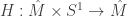
OK, let’s begin to discuss the content of Mess’ paper. We can assume by passing to a cover if necessary that M is a closed, oriented 3-manifold whose fundamental group contains a central Z subgroup. For simplicity, let’s in fact assume that the center is actually equal to Z; it is easy (modulo facts well-known at the time) to reduce to the case that the center has rank 1, but it is subtle to deal with the possibility that the center might be infinitely generated. In any case, the first main theorem Mess proves (corresponding to Theorem 1, page 2) is:

Theorem: Let M be closed, irreducible, orientable. Suppose that center is Z. Then the covering space with fundamental group equal to this center is homeomorphic to a solid torus.

This is proved by “bare hands”, so to speak. Let’s let denote the generator of the center. Because it is central, the element is well-defined as an element of for any point p, so we can build (e.g. inductively on the skeleta of a triangulation) a homotopy such that the track of every point in M under the homotopy is in the class of . We can lift this homotopy to ; because M was compact, the length of the tracks of the homotopy have uniformly bounded length. For homological reasons, is one-ended, and the first point is that every compact set K in can be separated from this end by an embedded torus T in such a way that is still central in , where E is the noncompact region bounded by T. To see this, first observe that K can be included in a big compact set K” such that the track of under the homotopy H stays disjoint from K (this uses the fact that the tracks themselves have uniformly bounded length). The surface is essential in , and its image under H sweeps out an immersed 3-manifold whose image G in contains a central Z subgroup (the image of the tracks of the homotopy). Pass to the cover of ; this manifold has nontrivial , and is therefore Haken, so (because it has a central Z subgroup) it was known to be a Seifert fibered space. Thus the surface can be replaced by a homologically equivalent embedded torus, which necessarily bounds a solid torus in . So is an increasing union of solid tori; a further standard argument shows that these tori nest nicely in each other, and the union is a solid torus.

Now, at this stage, has two useful structures: topologically it is homeomorphic to a solid torus , while geometrically it admits a homotopy whose tracks have bounded length. The next step is to find a relationship between these two structures:

Theorem: With as above, there is a homotopy whose tracks have uniformly bounded diameter, which starts at and ends at a free circle action on witnessing its topological product structure.

In words, J is a bounded homotopy from H to the Seifert structure. In particular, because J has fibers of bounded diameter, admits a product structure for which the circle fibers have uniformly bounded length. The homotopy J is constructed inductively out of “round handles” — i.e. products of circles with ordinary (2-dimensional) handles. First, we can pick any unknotted core of the solid torus, and take this to be the image of some track of H under the homotopy J. The deck group (which is a group because is central and therefore normal) acts on by isometries, and therefore by homeomorphisms; and thus permutes the set of positively oriented unknotted cores, since these are the only unknotted circles which represent homotopically. Choose a separated net in G — a collection of elements such that no two are very close, and such that every element is not too far away from something in the net. Evidently we can choose such a net so that the translates of by elements of the net are all mutually unlinked, and collectively represent an unknotted collection of circles in . Thicken each such circle to a round 0-handle; these will be the round 0-handles in our decomposition.

Building the round 1-handles is tricky, and requires quite an ingenious argument. Because we chose a separated net, every round 0-handle is close to some, but not too many, other round 0-handles. Any two round 0-handles which are close enough can be connected by some annulus (because their cores are isotopic), and we can least area representatives. Two such least area annuli cannot intersect on their boundaries (unless they agree), by the roundoff trick. Thus, any two of them will intersect transversely in finitely many essential circles. So we pick a starting 0-handle and inductively attach least area annuli one at a time, choosing the absolute smallest area one among the finitely many (up to isotopy) which join an unattached 0-handle (which we will call ) to one of the constructed so far, and by a roundoff argument, we see that the result is embedded. By transfinite induction, all the round 0-handles can be connected up in this way after some countable ordinal stage. The annuli we attach can be thickened to become round 1-handles, and the result is a tree of round 0-handles, connected up by round 1-handles, all with uniformly bounded diameter (this is because at every stage some yet to be connected is bounded distance from the union of the handles connected so far, so the annuli which are attached have uniformly bounded diameter).

Now consider a component X of the boundary of the union of round 0- and 1-handles constructed so far. Note that X is partitioned into annuli of bounded diameter which are on the boundaries of the o-handles, and which are on the boundaries of the 1-handles. They appear in a particular order . Adding further round 1-handles splits X into components, some of which might be bounded. We would like to add new annuli, to split X up into components of uniformly bounded (combinatorial) size; to do this, we need to find pairs of which are a uniformly big combinatorial distance apart, but which can be joined by and embedded annuli of uniformly bounded diameter. It is intuitively clear that this can be done: if X is noncompact, the two “ends” of X can’t get too far away from each other, or else there would be an arbitrarily big embedded ball contained in the complement, which is incompatible with the fact that we chose a separated net’s worth of translates of our original 0-handle. A similar argument works when X is compact but sufficiently big (alternately one can suppose not and take pointed limits, since this is a purely geometric argument). Thus we can attach round 1-handles of uniformly bounded diameter so that at the end, every component X itself has bounded diameter, and can be filled in with a round 2-handle. The construction of J with this handle decomposition as the end result is routine.

This brings us to section 3 of Mess’ paper (page 11), entitled, On groups which are coarse quasi-isometric to planes. The group in question is G, i.e. . This is the group that we hope will turn out to be the orbifold fundamental group of O, if the Seifert Conjecture is true. Since it is infinite, we want to show that G is a lattice in the group of isometries of the Euclidean or hyperbolic plane; in fact, a cocompact lattice, since M is closed. In particular, this should imply at least that G is quasi-isometric either to the Euclidean or the hyperbolic plane. By the Schwarz lemma, we know that G is quasi-isometric to , and we have constructed a product structure on whose fibers have uniformly bounded length. It is therefore straightforward (e.g. by averaging over fibers) to construct a complete Riemannian metric on the plane (which we denote P) so that G is quasi-isometric to P. The next main result is Theorem 7 (page 13) which says:

Theorem: Suppose a finitely generated group G is quasi-isometric to a plane P with a complete Riemannian metric. If P is conformally equivalent to the hyperbolic plane, then G is quasi-isometric to the hyperbolic plane.

Note that P has bounded geometry (i.e. 2-sided curvature bounds, and injectivity radius bounded below). One subtlety, observed by Mess, is that the plane admits complete Riemannian metrics with bounded geometry, and in the conformal class of the hyperbolic plane, but for which 0 is the bottom of the spectrum of the Laplacian; a group quasi-isometric to such a space would be amenable, by a famous theorem of Brooks, whereas no group quasi-isometric to the hyperbolic plane can be amenable. Nevertheless, there is a short-cut to proving this theorem, by invoking Candel’s theorem, alluded to above. Candel proves that if  L is a compact Riemann surface lamination all of whose leaves are conformally hyperbolic, then the leafwise uniformization map is continuous; in particular, since L is compact, the uniformization map is bilipschitz (and in particular is a quasi-isometry). Now, a Riemannian manifold with bounded geometry can be realized as a dense leaf in a lamination by taking its closure in pointed Gromov-Hausdorff space; if we do this to P, we obtain a lamination L. A priori a lamination can have leaves of different conformal type; see e.g. this post; but in this case P is uniformly quasi-isometric to G, and therefore (since G acts cocompactly on itself) the same must be true for every leaf of L. Now apply Candel’s theorem; qed. Mess’ argument is not especially hard to follow, but I believe that invoking Candel makes the situation clearer.

Finally we must deal with the case that P is quasi-isometric to the Euclidean plane. In this case, Theorem 10 (page 20) says (paraphrasing):

Theorem: Suppose is quasi-isometric to a plane P with a complete Riemannian metric, which is conformally equivalent to the Euclidean plane. Then G is virtually rank 2 abelian, and M is Seifert fibered; thus, the Seifert Fiber Conjecture holds in this case.

The argument is a beautiful application of ideas from the theory of random walks, combined with a theorem of Varopoulos. It is a well-known fact that a simple random walk is recurrent (i.e. returns to a bounded region infinitely often) in Euclidean space of dimension 1 and 2, and transient otherwise. This is not hard to show: under random walk on Euclidean space, after n steps each coordinate function is distributed like a Gaussian with variance of order n; thus the probability that a given coordinate function will be bounded by a constant C after n steps is of order . By independence, in m-dimensional space, the probability that all coordinate functions will be bounded by the same constant C at the same time after n steps is ; thus, when m is at least 3, the total number of times this should happen in an infinite walk is bounded, by the Borel-Cantelli Lemma. Now, in the continuum limit, a simple random walk rescales to Brownian motion, and Brownian motion is conformally invariant in dimension 2; this means that if you have a complete Riemannian metric on a plane P, you can tell whether it is conformally hyperbolic or conformally Euclidean by whether Brownian motion is transient or recurrent. Using the quasi-isometry between P and G, one concludes that if P is conformally Euclidean, random walk on G is recurrent. But this is an extremely confining possibility for finitely presented groups; Varopoulos showed (when combined with Gromov’s famous theorem that groups of polynomial growth are virtually nilpotent) that it implies that G is virtually abelian of rank at most 2; this is enough to complete the proof, using the (known) classification of nilpotent 3-manifold groups.

Mess’ paper thus reduces the Seifert Fibered Conjecture to the question of whether groups quasi-isometric to the hyperbolic plane are virtually isomorphic to Fuchsian groups — i.e. to (cocompact) lattices in the group of isometries of the hyperbolic plane. Much progress on this question had already been made by Tukia, and while Mess’ paper was still under consideration at JAMS (maybe in a sense it is still under consideration there?) this question was solved in the affirmative independently (and in quite different ways) by Casson-Jungreis, and Gabai (see the comments by Darryl linked to above).

Tastes change; fashions come and go even in mathematics. After Perelman proved the Geometrization Theorem, this story and the mathematical content of these papers faded somewhat into the background, to be quoted if necessary, but rarely read. Mess’ paper in particular — and especially its beautiful and original tone, style and ideas — is in danger of disappearing from our collective consciousness. Today when borrowing some books from the Crerar Library I noticed a Latin inscription: Non est mortuus qui scientiam vivificavit (translation: “He has not died who has given life to knowledge”). But knowledge can die too, and culture, and ideas. My life has been enriched by Geoff’s beautiful ideas, and I’m happy to do my bit to see that they, and maybe some of him, live on a little longer, enriching us all.

Riemannian manifolds are not primitive mathematical objects, like numbers, or functions, or graphs. They represent a compromise between local Euclidean geometry and global smooth topology, and another sort of compromise between precognitive geometric intuition and precise mathematical formalism.

Don’t ask me precisely what I meant by that; rather observe the repeated use of the key word compromise. The study of Riemannian geometry is — at least to me — fraught with compromise, a compromise which begins with language and notation. On the one hand, one would like a language and a formalism which treats Riemannian manifolds on their own terms, without introducing superfluous extra structure, and in which the fundamental objects and their properties are highlighted; on the other hand, in order to actually compute or to use the all-important tools of vector calculus and analysis one must introduce coordinates, indices, and cryptic notation which trips up beginners and experts alike.

Actually, my complicated relationship began the first time I was introduced to vectors. It was 1986, I was at a training camp for Australian mathematics olympiad hopefuls, and Ben Robinson gave me a 2 minute introduction to the subject over lunch. I found the notation overwhelming, and there was no connection in my mind between the letters and subscripts on one side of the page and the squiggly arrows and parallelograms on the other side. By the time the subject came up again a few years later in high school, somehow the mystery had faded, and the vocabulary and meaning of vectors, inner products, determinants etc. was crystal clear. I think that the difference this time around was that I concentrated first on learning what vectors were, and only when I had gotten the point did I engage with the question of how to represent them or calculate with them. In a similar way, my introduction to div, grad and curl was equally painless, since we learned the subject in physics class (in the last couple of years of high school) in the context of classical electrodynamics. I might have been challenged to grasp the abstract idea of a “vector field” as it is introduced in some textbooks, but those little pictures of lines of force running from positive to negative charges made immediate and intuitive sense. In fact, the whole idea of describing a vector field as a partial differential operator such as obscures an enormous complexity; it’s easy enough to compute with an expression like this, but as a mathematical object itself it is quite sophisticated, since even to define it we need not just one coordinate but an entire system of coordinates on some nearby smooth patch. Contrast this with the intuitive idea of a particle moving along a line of force, and being subjected to some influence which varies along the trajectory. I’m grateful to whoever designed the Melbourne high school science curriculum in the late 1980’s for integrating the maths and physics curricula so successfully.

A few years later, as an undergraduate at the University of Melbourne, I was attending Marty Ross’ reading group as we attempted to go through Cheeger and Ebin’s Comparison theorems in Riemannian geometry, and the confusion was back. Noel Hicks’ MathSciNet review calls this book a “tight, elegant, and delightful addition to the literature on global Riemannian geometry”, although he remarks that the “tightness of the exposition and a few misprints leave the reader with some challenging work”. Today I love this book, and recommend it to anyone; but at the time it was a terrible book to learn Riemannian geometry from for the first time (actually, since I was not a maths major, my confusion was amplified by many gaps in my intermediate education). Some aspects of the book I could appreciate — at least we were not drowning in indices, and the formulae were almost readable. But I was simply at a loss to understand the rules of the game — what sort of manipulations of formulae were allowed? how do you contract a vector field with a form? why am I allowed to choose coordinates at this point so that everything magically simplifies? how would anyone ever stumble on the formula for the Ricci curvature and see that it was invariant and had such nice properties? and so on.

And yet again, the duration of a couple of years made a world of difference. As a graduate student at Berkeley taking classes from Shoshichi Kobayashi and Sasha Givental, suddenly everything made sense (well, not everything, but at least the rudiments of Riemannian geometry). The difference again was that the notation and the calculations followed a discussion of what the objects were, and what information they contained and why you might want to use them or talk about them. And, crucially, this initial discussion was carried out first informally in words rather than by beginning with a formal definition or a formula.

So with this backstory in mind, I hope it might be useful to the graduate student out there who is struggling with the elements of the tensor calculus to go through a brief informal discussion of the meaning of some of the basic differential operators, which are the ingredients out of which much of the beauty of the subject can be synthesized.

Let’s get down to brass tacks. We start with a smooth manifold M and a vector field X. What is a vector field? For me I always think of it dynamically as a flow: the manifold is something like a fluid, and an object in M will be swept along by this flow and moved along the flowlines, or integral curves of the vector field. On a smooth manifold without a metric it doesn’t make sense to talk about whether the flow is moving “fast” or “slow”, but it does make sense to look at the places where it is stationary (the zeros of the vector field) and see whether the zeros are isolated or not, stable or unstable, or come in families. If f is a smooth function on M, the value of f varies along the integral curves of the vector field, and we can look at the rate at which the value changes; this is the derivative of f in the direction X, and denoted Xf. It is a smooth function on M; we can iterate this procedure and compute X(Xf), X(X(Xf)) and so on. The level sets of a smooth function f are (generically) smooth manifolds, and the whole idea of calculus is to approximate smooth things locally by linear things; thus generically through most points we can look at the level set of f through that point, and the tangent space to that level set. This is a hyperplane, and is spanned locally by the vector fields for which Xf is zero at the given point. More precisely, we can define a 1-form df just by setting df(X) = Xf; where df is nonzero, the kernel of df is the tangent space to the level set to f as described above.

Grad. Now we introduce a Riemannian metric, which is a smooth choice of inner product on the tangent space at each point. It does two things for us: first, it lets us talk about the speed of a flow generated by a vector field X (or equivalently, the size of the vectors); and second, it lets us measure the angle between two vectors at each point, in particular it lets us say what it means for vectors to be perpendicular. If f is a smooth function on a Riemannian manifold, we can do more than just construct the level sets of f; we can ask in which direction the value of f increases the fastest (and we can further ask how fast it increases in that direction). The answer to this question is the gradient; the gradient of f is a vector field which points always in the direction in which f increases the fastest, and with a magnitude proportional to the rate at which it increases there. In terms of the level sets of the function f, any vector field can be decomposed into a part which is tangent to the level sets (this is the part of the vector field whose flow keeps f unchanged) and a part which is perpendicular to it; the gradient is thus everywhere perpendicular to the level sets of f.

The inner product lets us give isomorphisms between vector fields and 1-forms called the sharp and flat isomorphisms. If is a 1-form, and X is a vector field, we define the vector field and the 1-form by the formulae

and

Sharp and flat are inverse operations. In words, a vector field and a 1-form are related by these operations if at each point they have the same magnitude, and the direction of the vector field is perpendicular to the kernel of the 1-form (i.e. the tangent space on which the 1-form vanishes). Using these isomorphisms, the gradient of a function f is just the vector field obtained by applying the sharp isomorphism to the 1-form df. In other words, it is the unique vector field such that for any other vector field X there is an identity

The zeros of the gradient are the critical points of f; for instance, the gradient vanishes at the minimum and the maximum of f.

Div. In Euclidean space of some dimension n, a collection of n linearly independent vectors form the edges of a parallelepiped. The volume of the parallelepiped is the determinant of the matrix whose columns are the given vectors. Actually there is a subtlety here — we need to choose an ordering of the vectors to take the determinant. A permutation might change the determinant by a factor of -1 if the sign of the permutation is odd. On an oriented Riemannian n-manifold if we have n vectors at a point, we can convert them to 1-forms and wedge them together — the result is an n-form. On an n-dimensional vector space, any two n-forms are proportional. Wedging together the 1-forms associated to a basis of perpendicular vectors of length 1 (an orthonormal collection) gives an n-form at each point which we call the volume form, and denote it . For any other n-tuple of vectors the volume of the parallelepiped is equal to the ratio of the n-form they determine (by taking sharp flat and wedging) and the volume form.

Now, there is an operator called Hodge star which acts on differential forms as follows. A k-form can be wedged with an (n-k) form to make an n-form, and this n-form can be compared in size to the volume form. We define the (n-k) form to be the smallest form such that

In other words, is perpendicular to the subspace of forms with . With this notation is the constant function equal to 1 everywhere; conversely for any smooth function f we have .

If X is a vector field, the flow generated by X carries along not just points, but tensor fields of all kinds. Covariant tensor fields are pushed forward by the flow, contravariant ones are pulled back. Thus a stationary observer at a point in M sees a one-parameter family of tensors of some fixed kind flowing through their point, and they may differentiate this family. The result is the Lie derivative of the tensor field, and is denote . The divergence of a vector field X measures the extent to which the flow generated by X does or does not preserve volume. It is a function which vanishes where the field infinitesimally preserves volume, and is biggest where the flow expands volume the most and smallest where the flow compresses volume the most.

The Lie derivative of the volume form is an n-form; taking Hodge star gives a function, and this function is the divergence. Thus:

In terms of the operators we have described above, applying flat to a vector field X gives a 1-form . Applying Hodge star to this one form gives rise to an (n-1)-form, then applying d gives an n-form, and this n-form (finally) is precisely . Thus,

Gradient and divergence are “almost” dual to each other under Hodge star, in the following sense. Let’s suppose we have some function f and some vector field X. We can take the gradient and form , and then we can look at the inner product of the gradient with X to obtain a function, and then integrate this function over the manifold. I.e.

But

If M is closed, the integral of an exact form over M is zero, so we deduce that

so that -div is a formal adjoint to grad.

Laplacian. If f is a function, we can first apply the gradient and then the divergence to obtain another function; this composition (or rather its negative) is the Laplacian, and is denoted . In other words,

Note that there are competing conventions here: it is common to denote the negative of this quantity (i.e. the composition div grad itself) as the Laplacian. But this convention is also common, and has the advantage that the Laplacian is a non-negative self-adjoint operator. The Laplacian governs the flow of heat in the manifold; if we imagine our manifold is filled with some collection of microscopic particles buzzing around randomly at great speed and carrying kinetic energy around, then the temperature is a measure of the amount of energy per unit of volume. If the temperature is constant, then although the particles can move from point to point, on average for each particle that moves out of a small box, there will be another particle that moves in from the outside; thus the ensemble of particles is in “thermal equilibrium”. However, if there is a local hot spot — i.e. a concentration of high energy particles — then these particles will have a tendency to spread out, in the sense that the average number of particles that leave the small hot box will exceed the number of particles that enter from neighboring cooler boxes. Thus, heat will tend to spread out by the vector field which is its negative gradient, and where this vector field diverges, the heat will dissipate and the temperature will cool. In other words, if f is the temperature, then the derivative of temperature over time satisfies the heat equation . Actually, since heat can come in or out from any direction, what is important is how the heat at a point deviates from the average of the heat at nearby points. The stationary heat distributions — i.e. the functions f with — are therefore the functions which satisfy an (infinitesimal) mean value property. These functions are called harmonic.

The erratic motion of the infinitesimal particles as they bump into each other and drift around is called Brownian motion, after the botanist Robert Brown, who is known to Australians for being the naturalist on the scientific voyage of the Investigator which sailed to Western Australia in 1801. Later, in 1827, he observed the jittery motion of minute particles ejected from pollen grains, and the phenomenon came to be named after him. Thus, a function on a Riemannian manifold is harmonic if its expected value stays constant under random Brownian motion, and the Laplacian describes the way that the expected value of the function changes under such motion.

Curl. After converting a vector field to a 1-form with the flat operator, one can apply the operator d to obtain a closed 2-form. On an arbitrary Riemannian manifold, this is more or less the end of the story, but on a 3-manifold, applying Hodge star to a 2-form gives back a 1-form, which can then be converted back to a vector field with the sharp operator. This composition is the curl of a vector field; i.e.

Notice that this satisfies the identities

and

Thus one of the functions of the curl operator is to give a necessary condition on a vector field to arise as the gradient of some function; such a function, if it exists, is called a potential for the vector field. Since a gradient flows from places where the function is small to where it is large, it does not recur or circulate; hence in a sense the curl measures the tendency of the vector field to circulate, or to form closed orbits. Actually there is a subtlety here which is that the curl will vanish precisely on vector fields which are locally the gradient of a smooth function. The topology of M — in particular its first homology group with real coefficients — parameterizes curl-free vector fields modulo those which are gradients of smooth functions.

As mentioned above, the curl measures the tendency of the vector field to spiral around an axis (locally); the direction of this axis of spiraling is the direction of the vector field , and the magnitude is the rate of twisting. Another way to say this is that the magnitude of the curl measures the tendency of flowlines of the vector field to wind positively around each other. A vector field and its curl can be proportional; such vector fields are called Beltrami fields and they arise (up to rescaling) as the Reeb flows associated to contact structures.

On an arbitrary Riemannian n-manifold it is still possible to interpret the curl in terms of rotation or twisting. Using the sharp and flat isomorphisms, a 2-form determines at each point a skew-symmetric endomorphism of the tangent space. The endomorphism applies to a vector by first contracting it with the 2-form to produce a 1-form, then using the sharp operator to transform it back to a vector. The skew-symmetry of this endomorphism is equivalent to the alternating property of forms. Now, a skew-symmetric endomorphism of a vector space can be thought of as an infinitesimal rotation, since the Lie algebra of the orthogonal group consists precisely of skew-symmetric matrices. Thus a vector field X on a Riemannian manifold determines a field of infinitesimal rotations, and this field is one way of thinking of . On a 3-manifold, a rotation has a unique axis, and this axis points in the direction of the vector field . On a Kähler manifold, the Kähler form determines a field of infinitesimal rotations which rotate the complex directions at constant speed.

Strain. Actually, the curl, the divergence, and a third operator called the strain can all be put on a uniform footing, as follows. We continue to think of a vector field X as a flow on a smooth manifold M. Tensor fields are pushed or pulled around by X, and an observer at a fixed point sees a 1-parameter family of tensors (of a fixed kind) evolving over time. But we would like to be able to study the effect of X on an object which is carried about and distorted by the flow; for example, we might have a curve or a submanifold in M, and we might want to understand how the geometry of this submanifold is preserved or distorted as it is carried along by the flow. Calculus takes place in a fixed vector space, and the flow is moving our object along the flowlines. We need some way to bring the object back along the flowline to a fixed reference frame so that we can understand how it is being transformed by the flow. On a Riemannian manifold there is a canonical way to move tensor fields along flowlines: we move them by parallel transport. There is a unique connection on the manifold called the Levi-Civita connection  which preserves the metric, and is torsion-free. The first condition just means that parallel transport is an isometry from one tangent space to the other. The second condition is more subtle, and it means (roughly) that there is no “unnecessary twisting” of the tangent space as it is transported around (no yaw, in aviation terms). Think of a car moving down a straight freeway; the geometry of the car is (hopefully!) not distorted by its motion, and the occupants of the car are not unnecessarily rotated or twisted. When the car hits some ice, it begins to skid and twist; the occupants are still moved in roughly the same overall direction, and the geometry is still not distorted (until a collision, anyway), but there is unnecessary twisting — the “torsion” of the connection.

So on a Riemannian manifold, we can flow objects away by a vector field X, and then parallel transport them back along the flowlines with the Levi-Civita connection. Now “the same” tensor experiences the effect of the vector field X while staying in “the same” vector space, so that we can compute the derivative to determine the infinitesimal effect of the flow. This derivative is the operator denoted by Kobayashi–Nomizu, and it is easy to check that it is itself a tensor field for any fixed X, and therefore determines a section of the bundle of endomorphisms of the tangent bundle.

On a Riemannian manifold, the space of endomorphisms of the tangent space at each point is a module for the Lie algebra of the orthogonal group, and it makes sense to decompose an endomorphism into components which correspond to the irreducible factors. Said more prosaically, an endomorphism is expressed (in terms of an orthonormal basis) as a matrix, and we can decompose this matrix into an antisymmetric and a symmetric part. Further, the symmetric part can be decomposed into its trace (a diagonal matrix, up to scale) and a trace-free part.

In this language,

1. the divergence of X is the negative of the trace of ;
2. the curl of X is the skew-symmetric part of ; and
3. the strain of X is the trace-free symmetric part of .

The strain measures the infinitesimal failure of flow by X to be conformal. Under a conformal transformation, lengths might change but angles are preserved. The strain measures the extent to which some directions are pushed and pulled by the flow of X more than others; in general relativity, this is expressed by talking about the tidal force of the gravitational field. An extreme example of tidal forces is the spaghettification experienced (briefly) by an observer falling in to a black hole. In the theory of quasiconformal analysis, a Beltrami field prescribes the strain of a smooth mapping between domains.

and so on. This is a far from exhaustive survey of some of the key players in Riemannian geometry, and yet strangely I am temporarily exhausted. It is hard work to unpack the telegraphic beauty of Levi-Civita’s calculus into a collection of stories. And this is the undeniable advantage of the notational formalism — its concision. A geometric formula can (and often does) contain an enormous amount of information — much of it explicit, but some of it implicit, and depending on the reader to be familiar with a host of conventions, simplifications, abbreviations,  and even ad hoc identifications which might depend on context. Maybe the trick is to learn to read more slowly. Or if you have a couple of years to spare, you can always do what I did, and go away and come back later when the material is ready for you. For the curious, I have a few notes on my webpage, including notes from a class on Riemannian geometry I taught in Spring 2013, and notes from a class on minimal surfaces that I’m teaching right now (much of this blog post is adapted from the introduction to the latter). Bear in mind that these notes are not very polished in places, and the minimal surface notes are very rudimentary and only cover a couple of topics as of this writing.

I have tried to include at least one problem in each homework assignment which builds a connection between classical geometry and some other part of mathematics, frequently elementary number theory. For last week’s assignment I thought I would include a problem on the well-known connection between Pythagorean triples and the modular group, perhaps touching on the Euclidean algorithm, continued fractions, etc. But I have introduced the hyperbolic plane in my class mainly in the hyperboloid model, in order to stress an analogy with spherical geometry, and in order to make it easy to derive the identities for hyperbolic triangles (i.e. hyperbolic laws of sines and cosines) from linear algebra, so it made sense to try to set up the problem in the language of the orthogonal group , and the subgroup preserving the integral lattice in .

First, let’s recall the definition of the hyperboloid model of the hyperbolic plane. In we consider the quadratic form , and let denote the group of real matrices preserving this form. The vectors with are those lying on a 2-sheeted hyperboloid; the positive sheet H is the one consisting of vectors whose z coefficient is positive, and is the subgroup preserving this sheet. For each vector v in H, the tangent space is naturally isomorphic to the set of vectors with ; i.e. the subspace of vectors “perpendicular” to v with respect to the form. The restriction of the quadratic form to the tangent space is positive definite, so it makes H into a Riemannian manifold, in such a way that acts by isometries. This group acts transitively, and the stabilizer of a point is conjugate to ; thus H with this metric is homogeneous and isotropic, and is a model for the hyperbolic plane.

Another model is the upper half-space model of the hyperbolic plane. In this model, we define H to be the subspace of complex numbers with positive imaginary part, and let denote the group of real matrices, which acts on H by fractional linear transformations:

This action is not faithful; the subgroup acts trivially, so the action descends to the quotient . The group acts transitively, and the stabilizer of a point is conjugate to ; thus (again) H is homogeneous and isotropic, and is a model for the hyperbolic plane. This reflects the exceptional isomorphism of groups .

The subgroup acts discretely with finite covolume (i.e. it is a lattice in the Lie group ); the quotient is the modular surface — an orbifold with underlying surface a sphere with one puncture, and two cone points with order 2 and 3 respectively; one sometimes calls this the -triangle orbifold, since it is made from two semi-ideal hyperbolic triangles with angles at the vertices (the third “ideal” vertex is at infinity, and corresponds to the puncture). There is an associated tessellation of the hyperbolic plane by such triangles whose symmetry group is in which the ideal vertices lie exactly at the rational numbers (plus infinity) on the boundary of hyperbolic space. Thus acts in a natural way on the set of rational numbers union infinity, which can be thought of as the projective line over . As an abstract group, is the free product of two cyclic groups of order 2 and 3 respectively, corresponding to the matrices

   and    

and all torsion elements in are conjugate to these elements or their inverse (note that these matrices have orders 4 and 6 respectively in ; it is only in that they have orders 2 and 3).

The group is an example of what is known as an arithmetic lattice; roughly speaking, the arithmetic lattices in semisimple Lie groups G are those with “integer entries”, in a suitable sense.  Arithmetic lattices are characterized by the existence of many hidden symmetries — i.e. their finite index subgroups have surprisingly large normalizers in G. More formally, for a subgroup in G, we define the commensurator of to be the subgroup of G consisting of elements g such that the conjugate of by g intersects in a finite index subgroup. With this definition, Margulis famously proved that the arithmetic lattices are precisely those whose commensurators are dense, and that all other lattices (i.e. the non-arithmetic ones) have a commensurator which is discrete (and hence contains the lattice itself with finite index). In , all the arithmetic lattices are derived from quaternion algebras over totally real number fields. Roughly speaking, if is a totally real number field — i.e. a finite extension of obtained by adjoining some root of an integer polynomial with all real roots — and if is a quaternion algebra over , then we can find a group  consisting of “integer” elements of of norm 1. Each real embedding of embeds in a quaternion algebra over ; this is either the Hamiltonian quaternions (which is a division algebra), or the algebra of real matrices (which has zero divisors). Then embeds as a lattice in a product of copies of and , one for each real embedding in the Hamiltonian quaternions and in respectively. The factors are compact, so if there is exactly one factor, embeds as a lattice in it, and projects to a lattice in ; these are exactly the arithmetic lattices.

It is a theorem of Borel that the only way to get an arithmetic lattice in which is not cocompact is to take — in other words, .

OK, now — how to reproduce this picture in the hyperboloid model? The most natural guess is to look at — the group of matrices with integer entries preserving the quadratic form and the positive sheet of the hyperboloid. So, what exactly is this group? Let’s let A be a matrix in this group, and denote its column vectors by u,v,w. One obvious matrix to take is the identity matrix; for that matrix, the vector w is which lies on the hyperboloid H, whereas the vectors u and v are orthonormal vectors in . But this property of a triple of vectors is preserved by the action of any element of , and therefore in general there is a bijection between such matrices and triples u,v,w where w lies on H, and u,v are orthonormal vectors in .

Now consider the condition that the entries of the matrix be integers. Let’s abstract the discussion slightly. Suppose V is a real vector space of dimension n, with a symmetric nondegenerate quadratic form Q. Let L be a lattice in V; this is a slightly different use of the word “lattice” than above (at least in flavor) — it means a discrete cocompact additive subgroup, isomorphic as a group to . We suppose that the lattice L is integral and unimodular; the first condition means that is an integer for all in L, and the second means that the matrix with entries has determinant 1 or -1 for any basis of L. Now, for any nonzero vector the linear function has image of finite index (because Q is nondegenerate and L has full rank) and therefore the kernel has rank (n-1). If  has norm 1 or -1, then is itself an integral unimodular lattice in the vector space with respect to the quadratic form which is the restriction of Q.

In with the quadratic form Q as above, suppose we can find an integer vector w on the hyperboloid H. Then the intersection of  with the lattice of integer vectors has rank 2, and since the form Q is positive definite there, we can find an orthonormal basis u,v of integer vectors for . Hence there is a matrix A in taking to w, and acts transitively on such vectors, with stabilizer isomorphic to , the group of symmetries of the square. If we want to restrict attention to orientation-preserving symmetries, then is cyclic of order 4, generated by

Let’s find another matrix. An integral vector w on the hyperbolic H is a triple of integers x,y,z so that ; one simple example is , and then it is straightforward to find vectors and for u and v. This gives the matrix

Actually, it is pretty easy to see that no other integral vector on H is closer to than , since is not a sum of two squares. Let’s let be the group generated by R and T. Some experimentation with fundamental domains confirms that this group is a lattice, and that the quotient is a sphere with one puncture and two orbifold points of orders 2 and 4; in particular, this is the entire group , and its quotient is the triangle orbifold.

So, this group is certainly not . In fact, a rotation of order 4 realized as an element of necessarily has a trace of , so it can’t even have rational entries. But wait — this is surely an arithmetic lattice (for any conceivable definition of arithmetic), and therefore corresponds to some lattice derived from a quaternion algebra over a totally real number field. Since it is not cocompact, the only possibility is that the number field is , so that this lattice is commensurable with . At this point I vaguely recall something from a course on arithmetic lattices I took from Walter Neumann over 20 years ago in Melbourne, in which he stressed that the trace field of an arithmetic lattice (i.e. the field generated by the traces of the elements, thought of as a subgroup of ) is not by itself a commensurability invariant — rather the trace field generated by the squares of the elements is invariant; and the squares of the elements in this group all have integer trace after conjugating into . So mathematics is consistent after all, and I learn the surprising (to me) fact that the and triangle orbifolds are commensurable. Hard to believe I have been working with Kleinian groups for 20 years without noticing that before . . .

Here’s a picture of the tiling of the hyperbolic plane whose symmetry group is :

The center is the projection of and the adjacent 8-valent vertices are the projection of .

(Update May 20, 2014): As galoisrepresentations points out, the fact that the field generated by traces of squares of elements is a commensurability invariant is a theorem of Alan Reid.

This impression was dramatically shaken by Agol’s proof of the virtual Haken conjecture and virtual fibration conjectures in 3-manifold topology by an argument which depends for one of its key ingredients on the theory of non-positively curved cube complexes — a subject in geometric and combinatorial group theory which, while inspired by key examples in low-dimensions (especially surfaces in the hands of Scott, and graphs in the hands of Stallings), is definitely a high-dimensional theory with no obvious relations to manifolds at all. Even so, the transfer of information in this case is still from the “broad” world of group theory to the “special” world of 3-manifolds. It shows that 3-manifold topology is even richer than hitherto suspected, but it does not contradict the idea that the beautiful edifice of 3-manifold topology is an exceptional corner in the vast unstructured world of geometry.

I have just posted a paper to the arXiv, coauthored with Henry Wilton, and building on prior work I did with Alden Walker, that aims to challenge this idea. Let me quote the first couple of paragraphs of the introduction:

Geometric group theory was born in low-dimensional topology, in the collective visions of Klein, Poincaré and Dehn. Stallings used key ideas from 3-manifold topology (Dehn’s lemma, the sphere theorem) to prove theorems about free groups, and as a model for how to think about groups geometrically in general. The pillars of modern geometric group theory — (relatively) hyperbolic groups and hyperbolic Dehn filling, NPC cube complexes and their relations to LERF, the theory of JSJ splittings of groups and the structure of limit groups — all have their origins in the geometric and topological theory of 2- and 3-manifolds.

Despite these substantial and deep connections, the role of 3-manifolds in the larger world of group theory has been mainly to serve as a source of examples — of specific groups, and of rich and important phenomena and structure. Surfaces (especially Riemann surfaces) arise naturally throughout all of mathematics (and throughout science more generally), and are as ubiquitous as the complex numbers. But the conventional view is surely that 3-manifolds per se do not spontaneously arise in other areas of geometry (or mathematics more broadly) amongst the generic objects of study. We challenge this conventional view: 3-manifolds are everywhere.

3-Manifolds Everywhere Theorem: A random group, either in the few relators model or in the density model at any density less than 1/2, contains many quasiconvex subgroups isomorphic to the fundamental group of a compact hyperbolic 3-manifold with totally geodesic boundary.

The proof is direct — we basically show that one can directly construct a map from such a 3-manifold group into a random group (given by a random presentation) in such a way that it is very likely to be quasiconvex and injective. The argument borrows very heavily from many parts of my earlier paper with Alden, although the construction step is much more complicated.

It is possible to say something in general terms about the combinatorial construction. Our random presentation can be realized in geometric terms by building a 2-dimensional complex K, whose 1-skeleton X is a wedge of k circles (one for each generator), to which we attach disks along loops corresponding to the relators. Let r be one such relator; it is a long (cyclic) reduced word in the generators and their inverses. We can think of this word as being written along the edges of a circle L subdivided into intervals, with one letter in each interval. Imagine taking this circle and gluing it up to itself, matching sets of edges with the same label, so that the result is a labeled graph Z. If we then attach a disk along the boundary of the circle, we get a 2-complex M(Z), and this 2-complex immerses in K. If we are careful, we can arrange for M(Z) to have the homotopy type of a 3-manifold with boundary; and if the manifold is acylindrical and freely indecomposable with infinite fundamental group, it is the fundamental group of a compact hyperbolic 3-manifold with totally geodesic boundary.

Gluing up L to produce the “spine” Z so that M(Z) is homotopic to a 3-manifold is thus the bulk of the work. The spine Z will be a 4-valent graph, and the circle L will map to Z with degree 3 (i.e. every edge of Z has 3 preimages). At each vertex of Z, 6 edges in L run over the vertex in all possible ways from one incident edge of Z to another. The figure below shows three local models; the correct local model is the third one:

The key to the construction is to glue up collections of segments in L in triples, leaving a gap of three unglued segments of some fixed length which are the three edges of a theta graph (we call them “football bubbles”). Almost all the mass of L can be glued up this way, so we produce a reservoir of bubbles in a predictable distribution, and a remainder with relatively small mass. There are some operations that can then be performed on the remainder, gluing it up into the desired form, at the cost of adjusting the reservoir somewhat. Then the great mass of the reservoir is glued up into small disjoint collections whose local combinatorics can be completely specified; one particularly pretty move glues up four football bubbles (with suitably labeled edges) by draping them along the edges of a cube, each bubble aligned with one of the diagonal axes:

This idea of first performing a random matching which is “almost” right, which can then be adjusted at the cost of perturbing the distribution of an almost equidistributed “sea” of predictable pieces of bounded size, so that the rest of the matching decouples into a massive number of matching problems of uniformly bounded size that can be solved once and for all — is one that has come up in several places recently, including in the papers of Kahn-Markovic and my paper with Alden mentioned above, but also in Peter Keevash’s construction of General Steiner Systems and Designs (a paper  I learned of from Gil Kalai’s blog). This is an idea with remarkable power and potential, beyond the already impressive (but well-known) power of “random constructions”. And it shows that highly constrained and beautiful combinatorial and geometric objects — designs as well as 3-manifolds — can be built out of generic pieces.

So the purpose of this blog post is to advertise that I wrote a little piece of software called kleinian which uses the GLUT tools to visualize Kleinian groups (or, more accurately, interesting hyperbolic polyhedra invariant under such groups). The software can be downloaded from my github repository at

https://github.com/dannycalegari/kleinian

and then compiled from the command line with “make”. It should work out of the box on OS X; Alden Walker tells me he has successfully gotten it to compile on (Ubuntu) Linux, which required tinkering with the makefile a bit, and installing freeglut3-dev. There is a manual on the github page with a detailed description of file formats and so on.

One nice feature of the program is that the user just has to give semigroup generators for their (semi)-group, and a finite list of (hyperbolic) triangle orbits; the program then computes the Cayley graph out to some (user-specified) depth, applies the resulting set of transformations to the triangles, and renders the result. The code is available, and is licensed under the GPL, and I actively encourage anyone who wants to fork it and develop it into a more powerful tool to do so.

A few examples of output are:

universal cover of a genus 3 handlebody

universal cover of the fiber of the fibration of the figure 8 knot complement

space with Sierpinski carpet limit set invariant by super-ideal simplex reflection group

I wrote this program mainly just to produce some nice figures for a recent talk I gave at U Chicago to first-year graduate students; the talk itself can be downloaded from my webpage here. If you download this program, and enjoy using it, I would be very grateful to get feedback, or just to hear about your experience.

If X is a connected CW complex, by successively attaching cells of dimension 3 and higher to X we may obtain a CW complex Y for which the inclusion of X into Y induces an isomorphism on fundamental groups, while the universal cover of Y is contractible (i.e. Y is a with the fundamental group of X). The (co)-homology of Y is (by definition) the group (co)-homology of the fundamental group of X. Since Y is obtained from X by attaching cells of dimension at least 3, the map induced by inclusion is an isomorphism in dimension 0 and 1, and an injection in dimension 2 (dually, the map is a surjection, whose kernel is the image of under the Hurewicz map; so the cokernel of measures the pairing of the 2-dimensional cohomology of X with essential 2-spheres).

A surjective map f from a space X to a space S with connected fibers is surjective on fundamental groups. This basically follows from the long exact sequence in homotopy groups for a fibration; more prosaically, first note that 1-manifolds in S can be lifted locally to 1-manifolds in X, then distinct lifts of endpoints of small segments can be connected in their fibers in X. A surjection on fundamental groups induces an injection on in the other direction, and by naturality of cup product, if is a subspace of on which the cup product vanishes identically — i.e. if it is isotropic — then is also isotropic. If S is a closed oriented surface of genus g then cup product makes into a symplectic vector space of (real) dimension 2g, and any Lagrangian subspace V is isotropic of dimension g. Thus: a surjective map with connected fibers from a space X to a closed Riemann surface S of genus at least 2 gives rise to an isotropic subspace of of dimension at least 2.

So in a nutshell: the purpose of this blog post is to explain how the existence of isotropic subspaces in 1-dimensional cohomology of Kähler manifolds imposes very strong geometric constraints. This is true for “ordinary” cohomology on compact manifolds, and also for more exotic (i.e. ) cohomology on noncompact covers.

1. Fibered Kähler groups

For a compact Kähler manifold Hodge theory gives

(recall that the notation means the holomorphic p-forms). In other words, every (complex) 1-dimensional cohomology class has a unique representative 1-form which is a linear combination of holomorphic and anti-holomorphic 1-forms. Since the wedge product of holomorphic 1-forms is holomorphic (the first miracle mentioned in the previous post!), for holomorphic 1-forms we have

if and only if as forms. 

This has the following classical application:

Theorem (Castelnuovo-de Franchis): Let M be a compact Kähler manifold, and let V be a subspace of the space of holomorphic 1-forms on M which is isotropic with respect to the pairing (on cohomology; but equivalently, on forms). Suppose that the dimension of V is at least 2. Then there exists a surjective holomorphic map f with connected fibers from M to a compact Riemann surface C of genus g such that V is pulled back by f from C.

Proof: Let where be a basis of V. Where two forms don’t vanish, the condition that says that they are proportional, and therefore the ratio is a holomorphic function. If we let U denote the open (and dense) subset of M where none of the vanish, then the ratios define the coordinates of a holomorphic map to . Since is closed, its kernel is tangent to a (complex) codimension 1 foliation on U. Since the are closed, the ratio is constant on the leaves of , so the image of U in is 1-dimensional, and the map factors through a map to a compact Riemann surface D.

A priori a holomorphic map to a Riemann surface defined on an open set U does not extend to M; the simplest example to think of is the holomorphic function

where x and y are the two coordinate functions. This map is well defined away from the origin, where it is indeterminate. On the other hand, as we approach the origin radially along a (complex) line, the ratio is constant; so the map, defined on , extends over a copy of obtained by blowing up the origin. In general therefore a map extends to where M’ is obtained from M by blowing up along the indeterminacy of the map f, and the fibers of the blow-up map from M’ to M are all copies of .

Now, the map does not necessarily have connected fibers, but it is proper. So there is a (so-called) Stein factorization for some intermediate compact Riemann surface C, where has connected fibers, and is finite-to-one. As a set, the points of C are just the connected components of the point preimages of . As a complex manifold, the charts on are modeled on the transverse holomorphic structure on the foliation . Notice that since (as remarked above) the 1-forms are all locally constant on the leaves of , they descend to well-defined 1-forms on (which pull back to the under the map). In particular, we deduce that has genus at least . But now we see that there was no indeterminacy at all, since the fibers of the blow up admit no non-constant holomorphic map to a surface of positive genus, and therefore the map factors through after all. qed

Now suppose M is a compact Kähler manifold, and let V be a subspace of which is isotropic with respect to cup product, and of dimension at least 2. We can choose real harmonic 1-forms which are a basis for V, and take their holomorphic (1,0)-part .  Then is holomorphic, and is equal to the (2,0)-part of . Since the holomorphic 2-forms inject into cohomology, it follows that as forms. It is straightforward to check that the are linearly independent if the are, so we obtain an isotropic subspace of holomorphic 1-forms of the same dimension as V. Applying Castelnuovo-de Franchis, we see that M fibers over D as above (this observation is due to Catanese).

From this we easily deduce the following theorem of Siu-Beauville, proved originally by hard analytic methods (i.e. the theory of harmonic maps):

Corollary (Siu, Beauville): Let M be a compact Kähler manifold, and let . Then there is a holomorphic map with connected fibers from M to a compact Riemann surface C of genus at least g if and only if there is a surjective homomorphism .

Proof: A surjective map with connected fibers is surjective on fundamental groups. Conversely, a surjective map on fundamental groups pulls back injectively, and pulls back a maximal isotropic subspace of (which has dimension ) to an isotropic subspace of . qed

Definition: A Kähler group is fibered if it surjects onto the fundamental group of a compact Riemann surface of genus at least 2; equivalently, if some (equivalently: every) compact Kähler manifold with that fundamental group holomorphically fibers over a compact Riemann surface of genus at least 2 with connected fibers.

Note that the condition of being fibered implies .

2. L2 cohomology

Perhaps the fundamental method in geometric group theory is to study a group via its cocompact isometric action on some (typically noncompact) space. If G is the fundamental group of a manifold M, then G acts as a deck group on the universal cover of M. The aim of geometric group theory is to perceive algebraic properties of the group G in the “global” geometry of this universal cover.

The most important tool for the study of differential forms on compact Riemannian manifolds is Hodge theory. To use this tool on noncompact manifolds one must impose additional (global) restrictions on the forms that one studies. Thus Hodge theory on noncompact manifolds is related directly not to ordinary cohomology, but to more refined, quantitative versions, of which one of the most important is -cohomology.

If M is a smooth Riemannian manifold (not assumed to be compact), the pointwise inner product on forms gives rise to a global inner product which is well-defined on compactly supported forms. We say that a smooth form is in if

Now, the -forms do not usually form a chain complex, but we can pass to a subcomplex consisting of forms for which both and are -forms. Since this is a complex, and we can define cohomology:

 In general, the image of d is not a closed subspace (in the topology), so we define the reduced cohomology to be:

The advantage of working with reduced cohomology is that there is an -analogue of the Hodge theorem. The operators and still make sense on a noncompact Riemannian manifold, and so does . We can define the harmonic forms to be those for which , and we denote by the space of harmonic p-forms which are .

Let’s impose some reasonable global conditions on our manifold M. We say that a (complete) Riemannian manifold has bounded geometry if it satisfies the following two conditions:

1. The curvature and its derivatives satisfy uniform 2-sided bounds: for each k; and
2. The injectivity radius satisfies a uniform lower bound: everywhere.

Bounded geometry is the natural condition to impose to ensure that the manifold is “precompact” in Gromov-Hausdorff space; i.e. that for any sequence of points in the sequence of pointed metric spaces contain a subsequence which converge on compact subsets to a pointed Riemannian manifold . An equivalent way to think about it is that this is the condition which ensures that the Riemannian manifold can appear as a leaf in a compact lamination. The condition of bounded geometry is automatically satisfied for any cover (infinite or not) of a compact Riemannian manifold. Since this is essentially the only class of noncompact Riemannian manifolds we will consider, we hereafter assume that all our noncompact Riemannian manifolds have bounded geometry.

Theorem (L2 Hodge theorem): Let M be a complete Riemannian manifold with bounded geometry. Then every cohomology class in has a unique representative minimizing . Such a form is harmonic; i.e. it is in . Moreover, there is an orthogonal decomposition

One subtlety is that it is no longer true that is a formal adjoint to d, since integration by parts gives rise to a potentially nontrivial boundary term “at infinity”. But for an form , this boundary term vanishes, and one has

(since a priori the forms and are not , one first interprets this by using cutoff functions, and passing to a limit). In other words, a harmonic form which is also is closed and coclosed; conversely, any form which is closed and coclosed is harmonic (with no analytic conditions).

On a Kähler manifold the identity still holds pointwise (since this is a consequence purely of the local properties of the metric), and so there is a further decomposition of into components which are individually harmonic. There is furthermore a Hodge decomposition

and an form satisfies if and only if and . Thus consists precisely of holomorphic p-forms.

Example: A harmonic form which is not does not have to be in the kernel of d. For instance, a function is closed if and only if it is (locally) constant, but any nonconstant holomorphic function on a domain in has harmonic real and imaginary parts. On the other hand, suppose that is harmonic and , and exact as a form, so that for some smooth function f. Then we claim that f is actually harmonic (but not closed unless ). For, and commute, so is a constant c, and by the Gaffney cutoff trick, it can be shown that c=0.

3. Kähler hyperbolicity

Gromov showed that under certain geometric conditions, the reduced cohomology of a Kähler manifold vanishes outside the middle dimension. To define this condition, one first introduces the notion of a bounded form; this is a form for which is finite, where denotes the (operator) norm of at the point p.

Definition: A compact Kähler manifold M is Kähler hyperbolic if the pullback of the symplectic form to the universal cover satisfies for some bounded 1-form .

Suppose M is Kähler hyperbolic, and let be any harmonic form on . Then is closed, and

Since is bounded, the form is . On the other hand, is bounded (because it is pulled back from a form on a compact manifold), so is . Now, (recalling the notation L for the operation of wedging with the Kähler form), the Kähler identity is a purely local calculation, and therefore on any Kähler manifold (compact or not), wedge product with the Kähler form takes harmonic forms to harmonic forms. It follows that is harmonic, , and equal to the image of an form under d; thus it vanishes identically.

But if V is a real vector space of dimension 2n, and is a nondegenerate 2-form on V, then wedging with is injective on below the middle dimension (this is the linear algebra fact which underpins the Hard Lefschetz Theorem for compact Kähler manifolds). Thus the operator L is injective on harmonic -forms below the middle dimension. Dualizing, the operator is injective above the middle dimension, and we deduce the following:

Theorem (Gromov): If M is compact and Kähler hyperbolic, the reduced cohomology of the universal cover vanishes outside the middle dimension.

Example: If M is any compact manifold with then for any closed form on M the pullback of to the universal cover is d of a bounded form. This is proved by the Poincaré Lemma, since for a complete simply-connected manifold with , coning a submanifold along geodesics to a point gives a cone whose volume is bounded by the volume of the submanifold times a constant. So every Kähler manifold with a metric of strict negative curvature is Kähler hyperbolic. More generally, if M is merely nonpositively curved, and the flat planes are isotropic for the Kähler form, then the manifold is still Kähler hyperbolic. This applies (for example) to Kähler manifolds which are compact and locally symmetric of noncompact type. Generalizing in another direction, if M is Kähler with and word-hyperbolic, then M is Kähler hyperbolic.

4. Calibrations

The previous section shows that vanishes whenever M is Kähler hyperbolic of complex dimension at least 2, where denotes the universal cover of M. In fact, it turns out that one can completely understand the fundamental groups of Kähler manifolds for which  is nonzero: it turns out that such groups are always virtually equal to the fundamental group of a closed Riemann surface of genus at least 2.

So let’s suppose M is a compact Kähler manifold, that is its universal cover, and let’s suppose that  is nonzero. Since is simply-connected, every harmonic form (which is necessarily closed) is actually exact. Let be a nonzero harmonic form, and let denote its (1,0)-part, which is an holomorphic 1-form. Since is also exact, we can write for some holomorphic function on . By the coarea formula we compute

or in other words, most of the level sets have finite volume. On the other hand, these level sets are complete holomorphic submanifolds, and holomorphic submanifolds of Kähler manifolds turn out to enjoy a very strong geometric property, which we now explain.

On a Kähler manifold, the symplectic form is a calibrating form. This means that it satisfies the following two properties:

1. it is closed; and
2. it satisfies a pointwise estimate for all real 2k-planes A, with equality if and only if A is a complex subspace.

It follows that if S is a holomorphic submanifold of complex dimension k, and S’ is a real 2k dimensional submanifold obtained from S by a compactly supported variation so that S and S’ are in the same (relative) homology class, there is an inequality

In other words, holomorphic submanifolds of Kähler manifolds are absolute volume minimizers in their homology classes (amongst compactly supported variations). From this one deduces the following:

Lemma: Let M be a Kähler manifold with bounded geometry. Then for each k there is a constant C so that if S is a complete holomorphic submanifold of complex dimension k, there is an estimate

Proof: It suffices to show that for some fixed (taken to be the injectivity radius, say), there is a constant so that the volume of is at least for any point p in S. A Kähler manifold with bounded geometry is uniformly holomorphically bilipschitz to flat in balls of size smaller than the injectivity radius, so we need only prove this estimate for holomorphic submanifolds of .

But actually, the estimate follows just from the fact that S is a minimal surface. If S is a complete minimal surface of real dimension N in a Euclidean space, passing through the origin (say), then the Monotonicity Formula says that for any there is an inequality

This can be proved directly by using the vanishing of the mean curvature, but there is a softer proof that where C is the volume of the unit ball in Euclidean N dimensional space, which is enough for our purposes. To see this, observe that C is the limit of as R goes to zero. Suppose on some interval that somewhere, WLOG achieving its minimum at . The value of on gives a lower bound for the volume of , by the coarea formula. But the cone on evidently has less volume than this, in violation of the fact that S is calibrated. The estimate, and the proof follow. qed

It follows from this estimate that some of the fibers of are compact. The components of these fibers are the leaves of a foliation, and since the foliation is defined locally by a closed 1-form, the set of compact leaves is open; but these leaves are all locally homologous and thus have locally constant volume and therefore uniformly bounded diameter, so the set of compact leaves is closed, and therefore every leaf is compact. The space of leaves is 1 (complex) dimensional, and we thereby obtain a proper holomorphic map with connected fibers to a Riemann surface S. Note that the group of holomorphic automorphisms of (which includes the deck group ) must permute leaves of the foliation; for, since the leaves are compact, if their image were not contained in a leaf, the map to would be nonconstant, in contradiction of the fact that a holomorphic map from a compact holomorphic manifold to a noncompact one must be constant.

In summary, the deck group acts on permuting the fibers of the map h, and thus descends to an action on S. Because the fibers have uniformly bounded diameter, and the action of the deck group on is cocompact and proper, the action on S is also cocompact and proper. Since the map h is surjective with connected fibers, S is simply-connected; since the reduced -cohomology class is pulled back from S, it follows that S is the unit disk, and therefore contains a finite index subgroup which acts freely, and is isomorphic to the fundamental group of a closed Riemann surface of genus at least 2.

Now, it turns out that for a compact manifold M, the 1-dimensional -cohomology of the universal cover depends only on the fundamental group G of M, and is equal to , where the (reduced) cohomology groups may be defined directly from the bar complex. We have therefore proved the following theorem of Gromov:

Theorem (Gromov): Let G be a Kähler group with . Then G is commensurable with the fundamental group of a closed Riemann surface of genus at least 2.

5. Ends

To apply Gromov’s theorem (and its generalizations) it is important to have some interesting examples of groups with . Let X be a locally compact topological space. Then for every compact set K we have the set of components of X-K, and an inclusion induces . The space of ends of X (introduced by Freudenthal) is the inverse limit:

taken with respect to the directed system of complements of compact subsets. If each is finite, the space of ends is compact.

Now, let G be a finitely generated group. For each finite generating set we can build a Cayley graph C, which has one vertex for each element of G, and one edge for each pair of elements which differ by (right) multiplication by a generator. The graph C is locally finite and connected, and we define the space of ends of G, denoted , to be just . It turns out that this does not depend on the choice of a finite generating set, but is really an invariant of the group.

The theory of ends of groups is completely understood, thanks to the work of Stallings:

Theorem (Stallings, ends of groups): Let G be a finitely generated group. Then has cardinality 0,1,2 or . Moreover,

1. if and only if G is finite;
2. if and only if G is virtually equal to ; and
3. if and only if G splits as a nontrivial amalgam or HNN extension or where B is finite, and G is not virtually cyclic.

Actually, the only hard part of this theorem is the third bullet; the rest is elementary, and was known to Freudenthal. The third case is equivalent to the existence of a nontrivial action of G on a tree T (which is not a line) with finite edge stabilizers. It follows that groups with infinitely many ends are non-amenable.

Now, let M be a compact Riemannian manifold, and suppose that the fundamental group G has infinitely many ends. This implies that the universal cover also has infinitely many ends, and we may find a compact subset of whose complement has at least two unbounded regions. Define a function f on which is equal to 0 on some (but not all) of the unbounded regions of and 1 on the rest. Then has compact support (contained in K) and is therefore . On the other hand, if is any function with then is a constant, so is constant and nonzero on some end of , and is therefore not . It follows that is nonzero in unreduced .

Now, on functions f we have an equality . The Laplacian is self-adjoint, with non-negative real spectrum. So to prove that is equal to it suffices to establish a spectral gap for ; i.e. to prove an estimate of the form

for all functions f of compact support (which are dense in ).  In exactly this context one has the following famous theorem of Brooks:

Theorem (Brooks): with notation as above, one has  if and only if is an amenable group.

One can think of the size of as governing the rate of dissipation of the norm of a function f as it evolves by the heat equation . Geometrically it is plausible that heat dissipates at a definite rate when it is concentrated in a region whose boundary is big compared to its volume (since then a definite amount of heat can escape out the boundary). So heat should dissipate at a definite rate unless there are a sequence of compact regions in , exhausting , for which . To each such region one can assign a finite subset of G, by looking at which translates of a basepoint are contained in ; this sequence of subsets is known as a Følner sequence, and the existence of a Følner sequence for a countable group G is one of the definitions of amenability (the equivalence to the other standard definitions is due to Følner). The hard details of Brooks’ argument are to show that one can take subsets whose boundary is regular enough that the comparison between volumes of subsets and their boundaries in the continuous and the discrete world is uniform.

So in conclusion, if G is a group with infinitely many ends, then reduced and ordinary cohomology agree in dimension 1, and we can construct a nontrivial class as above. Putting this together we deduce the following:

Corollary (Gromov): A Kähler group is either finite, or has 1 end.

Proof: A group with two ends is virtually equal to , which is not Kähler because it has odd. A group with infinitely many ends has nontrivial reduced -cohomology in dimension one. But for a Kähler group, this implies the group is commensurable with the fundamental group of a closed surface of genus at least 2; such groups have only 1 end after all. qed

6. Ends and extensions

The arguments of Gromov can be generalized considerably. It should be remarked from the outset that at very few points in the proof of Gromov’s theorem did we use the fact that the manifold was the universal cover of M.

The following is proved by Arapura-Bressler-Ramachandran:

Theorem (Arapura-Bressler-Ramachandran):  Let M be a complete Kähler manifold with bounded geometry, and suppose that has dimension at least 2. Then there is a hyperbolic Riemann surface S and a proper holomorphic map with connected fibers. Moreover, the fibers of the map are permuted by the holomorphic automorphisms of M, and the map induces an isomorphism from  to .

Here the subscript “ex” means the harmonic 1-forms which are exact (as ordinary forms). Given an exact harmonic form we can take the holomorphic (1,0) part which is and closed. But we cannot assume it is exact if is nontrivial. If we only have one , then we are more or less stuck. But if we have at least two such forms, then the following remarkable Lemma (due originally to Gromov) applies:

Lemma (cup product): Let M be a complete Kähler manifold with bounded geometry, and let be real, harmonic exact 1-forms. Let be their (1,0)-components. Then pointwise.

Proof: The first remark to make is that on a complete Kähler manifold with bounded geometry, any harmonic form is actually bounded. Equivalently, since harmonic forms are smooth, there is no sequence of points going off to infinity such that the operator norms diverge. Since the manifold has bounded geometry, we can integrate the square of on disjoint balls of definite radius centered at such points, and the claim will therefore follow if we show the integral of the square of a harmonic form on a ball of definite radius is controlled by below by its value at the center. Assume we are in flat space; then this claim is obviously true for a linear form. But a harmonic form satisfies an elliptic 2nd order equation, which shows that the higher derivatives can be controlled in terms of the first derivative; the claim follows.

Now let be an exact harmonic form, and write . Suppose is a closed form. Then is in because is bounded (as above). If we define to be equal to f where and locally constant elsewhere, then is equal to where and vanishes elsewhere. But now is bounded, so is in , whereas in . We deduce that is zero in reduced cohomology.

Finally, if we let be the decomposition of the (1,0) forms into real and imaginary parts, then we compute

Now, the imaginary part of this is harmonic and ; on the other hand, we have just shown it is trivial in reduced cohomology. Thus it must vanish identically. But then must vanish identically too, proving the lemma. qed

It follows that the space  determines (by taking holomorphic parts) an isotropic subspace of , which by hypothesis has dimension at least 2. Each form in this space determines a complex codimension 1 foliation whose leaves are tangent to the kernel, and because the forms are closed and the space is isotropic, this foliation is independent of the choice of form. Furthermore, on any open subset where two such holomorphic 1-forms do not both vanish, the ratio defines a holomorphic map to .

At this point the following fact is extremely handy:

Proposition: Let M be a connected complex manifold (not assumed to be compact!) and and linearly independent closed holomorphic 1-forms with . Then has no indeterminacy; i.e. it defines a holomorphic map from M to .

This Proposition is Lemma 2.2 in a paper of Napier-Ramachandran, where they seem to suggest that the fact is standard, but give an elementary proof. Since the argument is local, one can write and and then one observes that the functions are locally constant on the fiber over each point ; the argument then follows essentially from a (co)dimension count.

Anyway, once this proposition is proved, it follows that the components of the level sets of this function agree with the leaves of , which can be taken to be the points of a Riemann surface S. An argument similar to the one above (using a pair of real harmonic functions instead of a single holomorphic function in the coarea formula) shows that some, and therefore every, leaf is compact of bounded volume. Pulling back an form on S gives something by uniform boundedness of the volume of the fibers; conversely, exact harmonic forms on M descend to S because they are constant on the leaves of the foliation. This proves the theorem.

Corollary: Let G be a Kähler group, and suppose there is an exact sequence

where and . Then H is commensurable to the fundamental group of a compact Riemann surface of genus at least 2.

Proof: Let M be a compact Kähler manifold with fundamental group G, and let N be the cover with fundamental group K. Then H acts on N cocompactly, and it follows that . An unbounded sequence of deck transformations must push most of the mass of an harmonic form off to infinity, so necessarily the space   is infinite dimensional; since is finite dimensional, there is an infinite dimensional space of exact forms. Thus N fibers over S as above. Since the map from N to S is surjective on fundamental groups, it follows that S is of finite type (because is finite dimensional). But the deck group H acts on S discretely and cocompactly by holomorphic automorphisms (which are isometries in the hyperbolic metric), so actually S is the disk. qed

Example (Arapura): The pure braid group surjects onto a (virtually) free group, with finitely generated kernel, and therefore it is never Kähler. Note that so these groups can’t always be ruled out as Kähler groups on the oddness of alone. On the other hand, pure braid groups are fundamental groups of hyperplane complements: the group is the fundamental group of the space of ordered distinct n-tuples of points in , which is the complement of a hyperplane arrangement in . So it follows that this quasiprojective variety can’t be compactified in such a way as that the compactifying locus has big codimension (or one could apply the Lefschetz hyperplane theorem).

 (Updated November 26: added references)

Based on this brief interaction, Volodya asked me to give a talk on the subject in the Geometric Langlands seminar. On the face of it, this was a ridiculous request, in a department that contains Kevin Corlette and Madhav Nori, both of whom are world experts on the subject of fundamental groups of Kähler manifolds. But I agreed to the request, on the basis that I (at least!) would get a lot out of preparing for the talk, even if nobody else did.

Anyway, I ended up giving two talks for a total of about 5 hours in the seminar in successive weeks, and in the course of preparing for these talks I learned a lot about fundamental groups of Kähler manifolds. Most of the standard accounts of this material are aimed at people whose background is quite far from mine; so I thought it would be useful to describe, in a leisurely fashion, and in terms that I find more comfortable, some elements of this theory over the course of a few blog posts, starting with this one.

This post is a gentle introduction to the (mostly local) geometry of Kähler manifolds themselves. Everything I say here is completely standard, and can be found in all the standard references (e.g. Griffiths and Harris; another very nice reference is Lectures on Kähler geometry by Moroianu). The main reason to go through this material so explicitly is to make transparent what parts of the theory still hold, and what need to be modified, when one considers the geometry of noncompact Kähler manifolds, especially those arising as (infinite) covering spaces of compact ones; but this point will need to wait to a subsequent post to be validated. The definition of a Kähler manifold has two parts: a linear algebra condition, and an integrability condition. We discuss these in turn.

1. Linear algebra

A Euclidean structure on V is just a positive definite symmetric inner product. After a change of basis, we can identify V with with its “standard” inner product (i.e. dot product). Thus the group of linear transformations of V preserving a positive definite symmetric inner product is isomorphic to the  orthogonal group .

A complex structure on V is just a linear endomorphism J which squares to -1. Since V is real, the eigenvalues of J are i and -i, each occurring with multiplicity equal to half the dimension of V (so the dimension of V had better be even). The endomorphism J extends by linearity to a complex-linear endomorphism of the complexification , where it becomes diagonalizable, and there is a canonical decomposition where V’ is the i-eigenspace, and V” is the -i-eigenspace of J. For any vector v in V there is a canonical decomposition

which we write as v = v’ + v”, where v’ is in V’ and v” in V”. The map from V to V’ taking v to v’ takes the operator J to multiplication by i, and identifies V with the complex vector space V’. Thus the group of (real) linear transformations of V preserving J is isomorphic to the complex linear group .

A symplectic structure on V is a non-degenerate antisymmetric inner product. This means a bilinear map satisfying , and such that for any nonzero v there is a nonzero w with . After a change of basis, we can identify V with  with its “standard” symplectic product; i.e. if we choose basis vectors then

, and

Thus the group of linear transformations of V preserving a symplectic form is isomorphic to the symplectic group .

Thus, a real vector space V of even dimension can admit a Euclidean structure, a complex structure, and a symplectic structure. These three structures are said to be compatible if they satisfy

for any two vectors v and w. Note that any two of these conditions implies the third. At the level of Lie groups, compatibility can be expressed in terms of the intersection of the stabilizers of the three structures:

1. ,
2. , and
3. 

Thus any two of the three structures (Euclidean, complex, symplectic) are compatible if the intersections of their stabilizers are isomorphic to a copy of the unitary group. The unitary group is the group of complex linear automorphisms of a complex vector space preserving a Hermitian form. This arises in the following way: a symmetric definite inner product on V induces a symmetric complex bilinear pairing on , and thereby a sesquilinear pairing H defined by

The restriction of H defines a Hermitian pairing on V’; identifying V’ with V gives a complex valued (real!) linear pairing on V whose real part is the given inner product, and whose imaginary part is the given symplectic form.

2. Integrability, and Kähler manifolds

Now let M be a real 2n-dimensional manifold. A Riemannian metric on M is a smoothly varying choice of positive definite inner product on the tangent spaces to M at each point. An almost complex structure is a smoothly varying choice of complex structure on the tangent spaces to M at each point. An almost symplectic structure is a smoothly varying choice of symplectic structure on the tangent spaces to M at each point. Expressed in terms of tensors, the Riemannian metric is a symmetric 2-form g, the almost complex structure is a section J of squaring to -1 pointwise, and the almost symplectic structure is an alternating 2-form .

The field of endomorphisms J determines a splitting of the complexification of T M into T’M and T”M pointwise. An almost complex structure is integrable if the bundle T’M is integrable; i.e. if the Lie bracket of two sections of this bundle is also a section of this bundle. Such a structure gives M the structure of a complex manifold, and is equivalent to the existence of an atlas of charts modeled on for which the transition functions between charts are holomorphic. An almost symplectic structure is integrable if the 2-form is closed; i.e. if as a form. Such a structure gives M the structure of a symplectic manifold, and is equivalent to the existence of an atlas of charts modeled on for which the transition functions between charts are symplectomorphisms (i.e. the derivative of the transition function at every point is a symplectic matrix).

Definition: A real 2n-manifold is Kähler if it admits a Riemannian metric, a complex structure, and a symplectic structure which are compatible at every point.

Every smooth manifold admits a Riemannian metric, and a manifold admits an almost complex structure if and only if it admits an almost symplectic structure (and either condition can be expressed in terms of properties of the characteristic classes of the tangent bundle). But the condition of integrability is much more subtle (at least for closed manifolds; any almost symplectic structure on an open manifold is homotopic to an integrable one).

Definition: A finitely presented group G is a Kähler group if it is equal to the fundamental group of a closed (i.e. compact without boundary) Kähler manifold.

Note that since the Kähler condition is preserved under taking covers and products, the class of Kähler groups is closed under passing to finite index subgroups, and taking (finite) products.

On any complex manifold we can choose coordinates locally so that the vector fields

are sections of T’M. The dual 1-forms and are a local basis for the smooth complex-valued 1-forms , and any complex 2-form can be expressed locally in the form

A Hermitian metric H determines such an h by 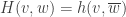; the Hermitian condition is equivalent to the symmetry of h (i.e. that ) and positivity (i.e. that is real and positive for all nonzero v). Any Riemannian metric on a complex manifold can be averaged under the action of J pointwise and then complexified and restricted to T’M to produce a Hermitian metric. Taking imaginary parts gives rise to an alternating 2-form

which is nondegenerate pointwise (i.e. is nowhere zero). The metric is Kähler if and only if .

Now, on a Riemannian manifold, one may always locally choose geodesic normal coordinates, centered at any given point, and in which the metric tensor g osculates the Euclidean metric (in these coordinates) to first order; i.e.

where O(2) denotes terms vanishing to at least 2nd order at the center. One way to find such coordinates is to take Euclidean coordinates on the tangent space at the center point, and push them forward by the exponential map. For a Hermitian metric on a complex manifold, one can choose holomorphic local coordinates with this property if and only if the metric is Kähler; that is,

Proposition: A Hemitian metric h on a complex manifold M is Kähler if and only if there are local holomorphic coordinates at any point for which

One direction of this proposition is easy: for such a choice of coordinates, the form is constant up to first order, and therefore at the given point. But the definition of exterior d is coordinate free, and therefore holds everywhere.

3. Dolbeault Cohomology

On any almost complex manifold M, the decomposition of the complexified tangent space into T’ and T” gives rise to a decomposition of its dual space, and we can decompose the space of complex-valued n-forms into components One coordinate-free way to see this decomposition is to extend the action of J on the (complexified) tangent space to an action of the circle (by complex linearity); this gives rise to an action of the circle on the complexified cotangent spaces, and to all its tensor powers. Thus the space of complex-valued n-forms decomposes into invariant subspaces for this circle action; the fiber of over each point is the subspace where acts as multiplication by .

If the almost complex structure is integrable, we can choose holomorphic coordinates locally, and then is spanned by forms

Thus (by differentiating in the usual way) we see that (this fact is equivalent to the integrability of the complex structure) and we can decompose d into and respectively, where and . These operators satisfy

So, for example, on a Kähler manifold, the symplectic form is both real (i.e. contained in ordinary ) and of type in .

Since , the various form a complex, whose homology groups are the Dolbeault cohomology, denoted . By analogy with the Poincaré lemma (which proves vanishing of ordinary de Rham cohomology of smooth manifolds locally) there is the Dolbeault Lemma, which says that any form with can be locally written as . This lets us take resolutions and compute cohomology; if we write for the sheaf of holomorphic p-forms (i.e. those forms which are in the kernel of ) then we obtain the

Dolbeault Theorem: for any complex manifold M, there is an isomorphism .

In particular, can be identified with the global holomorphic p-forms, which we denote (by abuse of notation) also by  .

From the Dolbeault Lemma one can also deduce the following:

Local  Lemma: if is a real 2-form of type , then if and only if we can write locally in the form for some real function .

If   is exact, such a function u can be found globally. When M is Kähler, the symplectic form can be expressed locally in the form ; such a function u is called a (local) Kähler potential. Conversely, every local potential u on a complex manifold for which the form  is nondegenerate (i.e. satisfies in its domain of definition) gives the manifold locally the structure of a Kähler manifold. Note that a Kähler potential cannot exist globally on a compact Kähler manifold.

4. Hodge theory

A Riemannian metric on a manifold induces inner products on the fibers of all natural bundles over the manifold, including the cotangent bundle and its tensor and exterior powers. On a Riemannian manifold of dimension n there is a Hodge star defined pointwise by

and we get an inner product on forms by .

The Hodge star operator satisfies the identity on k-forms. Define an operator from to for each k, and define the Laplacian to be the operator .

A form is harmonic if ; the harmonic p-forms are denoted . On any compact manifold there is a Hodge decomposition

where the summands are orthogonal. One deduces that there is an isomorphism , and that every (de Rham) cohomology class contains a unique harmonic representative, which is also the unique representative of smallest norm.

Again on a compact manifold, it turns out that is the formal adjoint of d with respect to the pairing on p-forms (for any p), and therefore that

One proves this by integration by parts, since the difference between the two sides differs by the integral of an exact form. Thus, a form is harmonic if and only if it is closed and coclosed (i.e. in the kernel of ).

On a complex manifold we extend Hodge star to complex-valued forms so that is the local Hermitian pairing. Thus . We can define formal adjoints

and Laplace operators

On a Kähler manifold, a surprisingly difficult local calculation gives the crucial identity

and therefore the (p,q) components of a harmonic p+q form are themselves harmonic!

Explicitly, we have a Hodge decomposition for (p,q)-forms using :

where are the (p,q)-forms in the kernel of , from which one deduces the Dolbeault isomorphism ; but from  one also gets the decomposition

One immediate miracle is the fact that on a Kähler manifold, holomorphic forms are harmonic. Explicitly, a (p,q)-form on a compact manifold is harmonic if and only if and . This follows from the identity

proved as before by integrating by parts. But for a (p,0) form, the operator is identically zero (since its image is in ), and a (p,0) form is in the kernel of if and only if it is holomorphic.

One reason to be impressed by this miracle is that the condition of being harmonic depends very delicately on the choice of a Riemannian metric, whereas the condition of being holomorphic depends only on the complex structure. Usually, the harmonic forms are only as regular as the metric; a Kähler metric is typically only smooth (one sees this by starting with one Kähler form and perturbing it by adding something of the form  for u a small bump function) whereas a complex structure is analytic. Anyway, this miracle has another miraculous consequence: since the wedge product of two holomorphic forms is holomorphic, it follows that the wedge product of two harmonic forms of type (p,0) and (q,0) is also harmonic, of type (p+q,0). As a rule of thumb, wedge products of harmonic forms (even on a Kähler manifold) is almost never harmonic, so this is an extraordinary fact.

Example: Let S be a closed Riemann surface of genus at least 2. There is a natural complex structure on S, and any Riemannian metric can be averaged under J to define a Hermitian metric, whose associated 2-form is automatically closed because S is 2-dimensional (as a real manifold). So S is Kähler. Let and be two real harmonic 1-forms which are not proportional; for instance, we could take to be the generator of . A real 1-form is dual to a vector field, and on a closed manifold, the number of singularities of a vector field (counted properly) is the Euler characteristic. Since , the forms and must be singular somewhere. This implies that must vanish somewhere; but the only (real) harmonic 2-form is the area form and its multiples, which does not vanish. Thus is never harmonic.

There are further symmetries of the various operators under consideration. Complex conjugation commutes with , so is isomorphic to . Similarly, the composition of Hodge star with complex conjugation commutes with , so is isomorphic to . If we denote the (complex) dimension of by , and the ordinary betti numbers of M by , we have identities

The last fact follows because the symplectic form and all its powers are real of type (p,p), and nontrivial in cohomology. In particular, notice that is even for k odd, and is positive for k even between 0 and 2n.

Example: finitely generated free groups are not Kähler, since they all have finite index subgroups with odd. The fundamental group of a Klein bottle is not Kähler, since it has ; on the other hand, this group has an index 2 subgroup which is Kähler (namely ).

5. Hard Lefschetz Theorem

One consequence of Hodge theory is so special it deserves to be singled out. Define an operator by (i.e. by wedging with the symplectic form). It has a formal adjoint ; in terms of an orthonormal basis it is defined by the formula (where denotes contraction — i.e. interior product). Define “twisted” operators

Then with these definitions one has the Kähler identities:

From this one can deduce another miracle: — in other words, the operators and descend to operators on . Notice as a special case that this implies the symplectic form is harmonic (it is not real analytic in general); actually this already follows from the fact that is closed, and so it is coclosed. More generally, the wedge product of the (harmonic) symplectic form with any harmonic form is harmonic.

The commutator acts on as multiplication by ; furthermore, it is elementary that and . Thus, the operators generate a copy of the Lie algebra , in a way which makes into a module over this Lie algebra. From the classification of finite dimensional modules, we deduce the:

Hard Lefschetz Theorem: The map is an isomorphism, and if we denote the kernel of by then . Furthermore, if we write the intersection of with by then .

Ordinary Poincare duality on a closed oriented 2n-manifold says that the pairing

is nondegenerate. Combining this with the Hard Lefschetz Theorem we deduce the Corollary:

Corollary: For all the pairing defined by

is nondegenerate.

The special case is particularly important; its nondegeneracy implies that the ordinary cup product cannot be too degenerate.

Example: if is the fundamental group of a closed surface of genus g, the universal central extension is not Kähler, since cup product on vanishes identically.

6. Holonomy

On any Riemannian manifold there is a unique connection on the tangent bundle called the Levi-Civita connection which is torsion-free, and which preserves the metric. This connection determines connections on the cotangent bundle and its tensor and exterior powers. If M is a complex manifold, and E is a holomorphic bundle on M with a Hermitian metric, any metric connection on M gives rise to connections ; decomposing the form part into types, there is a unique metric connection on E called the Chern connection whose (1,0) part is , when expressed in any local (holomorphic) coordinates.

The Kähler condition for a Riemannian metric on a complex manifold is equivalent to equality for the Levi-Civita connection and the Chern connection on the tangent bundle. This is equivalent to the condition that the tensors J and are parallel under (the Levi-Civita connection). Equivalently, the holonomy group of the metric is isomorphic to a subgroup of .

The coincidence of the Levi-Civita and Chern connections simplify the expression for the curvature of many natural bundles on a Kähler manifold. The most important example is the following. Let K be the canonical bundle on M (i.e.\/ the holomorphic line bundle whose holomorphic local sections are holomorphic n-forms where n is the dimension of M). Let denote the Ricci form on M; i.e. the real (1,1)-form defined by . Then the curvature of K (with its Hermitian metric arising from the Kähler metric on M) is equal to .

Some further remarks are in order:

1. The Kähler condition already implies that is a real alternating form of type (1,1), and since it is the curvature of a line bundle, it is automatically closed. So the local lemma says that it can be expressed locally in the form for some real u. In fact, if the coefficients of the Hermitian metric are given by (expressed in local coordinates), then .
2. Since the canonical bundle (as a holomorphic bundle, but ignoring its Hermitian metric) only depends on the complex structure, the form represents the first Chern class . Conversely, it is a famous theorem of Yau that on a Kähler manifold, for every 2-form representing the class there is a unique Kähler metric for which . As a corollary, M admits a Ricci-flat Kähler metric if and only if .
3. A Kähler metric is Ricci-flat if and only if the holonomy is a subgroup of . Such a manifold is the product (locally) of a flat manifold and compact pieces of complex dimension and with irreducible holonomy exactly equal to . These irreducible factors are called Calabi-Yau manifolds. A Calabi-Yau has a compact universal cover, and therefore its fundamental group is finite.

7. Weitzenböck formulae

Suppose is a “natural” second order elliptic operator on sections of a metric bundle E over a Riemannian manifold M. Naturality should mean that its symbol is invariant under the action of whatever orthogonal group acts in a structure preserving way on whatever bundle the symbol lies in. In many cases it is possible to take the square root of the symbol, and identify the square root as the symbol of some first-order operator D, so that and have the same (second-order) symbol. A priori one might expect the difference to be first order; but in many cases, the condition of naturality forces the first order term to vanish (because of the lack of an orthogonal group-invariant bundle map between and ). Thus the difference is a 0th order operator — i.e. a tensor. The only natural tensor fields on Riemannian manifolds are curvature fields, so we obtain a formula of the form

for some and some . If is in the kernel of , then by integrating we get

The integral of the first term is non-negative, and strictly positive unless vanishes. So if is a positive operator, the kernel of must be trivial. Such formulae are called (in this generality) Weitzenböck formulae, and the use of such formulae to prove triviality of the kernel of a natural elliptic operator under a curvature inequality is called the Böchner technique. There is a beautiful survey article on such formulae and their uses by Bourguignon.

Depending on the context, the operators might be more or less complicated. The simpler is, the more useful the formula.

Definition: a real (1,1)-form on a complex manifold is positive (resp. negative) if is positive definite (resp. negative definite). A cohomology class in is positive (resp. negative) if it can be represented by a positive (resp. negative) form. A holomorphic line bundle L is positive (resp. negative) if there is a Hermitian structure on L for which is positive (resp. negative) where is the curvature of the Chern connection

A line bundle is positive if and only if its first Chern class is positive (this can be proved by adjusting the curvature of the bundle by adjusting the metric, using the global form of the -Lemma).

Example: The Kähler form of a Kähler manifold is positive. The Ricci form of a Kähler manifold with positive Ricci curvature (in the usual sense) is positive. The canonical bundle of a Kähler manifold has curvature , so if the manifold has positive Ricci curvature, the canonical bundle is negative. For example, is Kähler with positive Ricci curvature (for the Fubini-Study metric), so its canonical bundle is negative. The dual of a positive line bundle is negative and vice versa, so every projective variety admits a positive line bundle (by restriction).

Kodaira applied a Weitzenböck formula to positive and negative holomorphic line bundles on compact complex manifolds, and proved the following vanishing result:

Proposition (Kodaira): Let L be a positive holomorphic line bundle on a compact Kähler manifold M. Then there is a positive integer so that for all and all .

From this one deduces the famous

Theorem (Kodaira embedding): If L is positive, then is arbitrarily large for all sufficiently large positive k. Consequently, a Kähler manifold is projective if and only if it admits a positive line bundle.

Proof: For any holomorphic bundle E, the holomorphic Euler characteristic

can be computed from the Atiyah-Singer index theorem by the formula

where Td is the Todd class, and ch is the Chern character, both formal power series in the Chern classes of the tangent bundle and of E respectively. All we need to know about the Todd class is that it starts with 1 in dimension 0. For a line bundle L we have

Since L is positive, is positive, and integrates over M to give a positive number. If k is big, this term dominates, and therefore is positive for all sufficiently big k. On the other hand, for all and all sufficiently big k, so we deduce that has arbitrarily many linearly independent holomorphic sections, when is big; in other words, L is ample. We obtain a projective embedding from ratios of these sections in the usual way. qed

(Appealing to the Atiyah-Singer index theorem is a cheap way to get nonvanishing of from vanishing of for ; Kodaira constructed his sections more directly, by building them locally, and then showing that the obstructions to patching the local sections together globally — which are parameterized by the higher — vanish.)

8. Lefschetz hyperplane theorem

If M is a (complex) n dimensional smooth projective variety in , its intersection V with a generic hyperplane H is smooth. The inclusion of V into M induces a map , and the classical statement of the Lefschetz hyperplane theorem says that this map is an isomorphism in dimensions and an injection in dimension .

In fact this statement about homology has a refinement at the level of homotopy, which can be proved by Morse theory, as observed by Bott.

Theorem (Lefschetz hyperplane): Let M be a complex n dimensional smooth projective variety, and let V be its intersection with a generic hyperplane. Then is an isomorphism for and is surjective for .

Bott showed how to build a Morse function on (converging to on ) such that at every critical point, the Hessian has at least n negative eigenvalues. In particular, M is obtained from V by attaching handles of dimension at least n, from which the theorem follows.

In particular, it follows that any group which can arise as the fundamental group of a smooth projective variety, can arise as the fundamental group of a smooth projective variety of complex dimension at most 2.

9. Examples of Kähler manifolds

Example (): the group acts projectively, holomorphically and transitively on , and the point stabilizers are conjugate to . Since point stabilizers are compact, it leaves invariant a Riemannian metric (unique up to scale), which is evidently compatible with the complex structure. The associated almost symplectic form is invariant under the group action, and easily seen to be parallel, and therefore the metric is Kähler. This is called the Fubini-Study metric. The Kähler “potential” on gives rise to a closed 2-form which is degenerate in radial directions, and descends to the Kähler form on . The curvature of the metric is pinched between 1 (in totally real directions) and 4 (in totally complex directions)

Example (nonsingular projective varieties): the Fubini-Study metric defines compatible complex and symplectic structures on every complex subspace of the tangent space at each point of , so it defines an almost Kähler structure on every holomorphic submanifold. The restriction of a closed form to a subspace is closed, so this structure is integrable. In the same vein, any holomorphic submanifold of a Kähler manifold is Kähler.

Example (bounded domains and their quotients): A bounded domain U in carries a canonical Hermitian metric, called the Bergman metric, which is invariant under all biholomorphic self-mappings of U. This is a Kähler metric, and descends to a canonical Kähler metric on any quotient . In fact, with respect to the Bergman metric, the canonical bundle is negative, and therefore (when is cocompact and acts without fixed points) the quotient  is projective (though not obviously so from the construction). Examples of bounded domains with a lot of symmetry are Hermitian symmetric spaces, so torsion-free cocompact lattices in groups like , , are Kähler groups.

Example (Riemann surfaces): Riemann surfaces are Kähler manifolds, and so are their products. Atiyah–Kodaira found examples of nontrivial algebraic surface bundles over surfaces, which can be obtained as branched covers of products over certain sections.

Example (): If M is any Kähler manifold with then M is actually projective. For, by symmetry, so . The Kähler form can be approximated by real harmonic 2-forms with rational periods, and by hypothesis, these nearby forms are of type (1,1). On the other hand, nearby forms are still positive, and because the periods are rational, after multiplying to clear denominators, the form is realized as the curvature of a (positive) line bundle.

Example (Voisin): Voisin found examples, in every complex dimension , of Kähler manifolds which are not homotopic to smooth projective varieties. However, these examples have free abelian fundamental groups, which are also fundamental groups of projective varieties.

 (Updated November 21: added several references)

Remember that a conformal map is one which infinitesimally takes round spheres to round spheres. That is, it is angle preserving, at least infinitesimally. In particular, it is smooth. So let’s think about a conformal map between open regions in Euclidean 3-space (for concreteness). The image of a flat plane P is a smooth surface f(P). Pick a point p in P and look at its image f(p). Infinitesimal round circles around p in P get taken to infinitesimal round circles around f(p) in f(P). And straight lines perpendicular to P get taken to smooth curves perpendicular to f(P). If you take a smooth surface S in Euclidean 3-space, and a small round circle in S, and push the circle off S in the perpendicular direction, some directions will be distorted more than others (typically): the infinitesimal circle gets distorted to an infinitesimal ellipse, whose major and minor axes are the directions of principal curvature on the surface S. But these ellipses are the conformal image of small round circles in the domain, and therefore should also be (almost) round. In other words: the principal curvatures at each point of f(P) should be equal. A point on a surface where the principal curvatures are equal is called an umbilical point, and a surface on which every point is umbilical is called totally umbilical.

It is a classical fact, proved by Meusnier in 1785, that an umbilical surface in Euclidean space is locally a piece of a plane or sphere. One way to see this is as follows. Let G denote the Gauss map, so that the condition of being umbilical at a point says exactly that dG is a multiple of the identity at that point (note: we are using here in the usual way the canonical identification between the tangent space to the surface and the tangent space to the round sphere at the image of the Gauss map at each point to think of dG as a map from the tangent space to itself). So if a surface is totally umbilical, there is some function f so that dG is equal to f times the identity at each point. Let’s denote by X a local chart on the surface giving rise to local coordinates u and v. So the definition of f says in this notation that and . But then

Since u and v are local coordinates, their tangent vectors and are independent, and therefore . This means that is (locally) constant. But this means that the surface osculates a sphere (or plane) of fixed curvature to first order at every point, and therefore (by developing this sphere along a path in the surface) the center of this osculating sphere is fixed and the surface agrees (locally) with the sphere (or plane). Incidentally, Gauss was only 8 years old in 1785, so whatever Meusnier’s proof was, he could not have mentioned the Gauss map by name. Does any reader know Meusnier’s argument?

Once we know that a conformal map takes subsets of planes and round spheres to subsets of planes and round spheres, we can intersect these planes and spheres with perpendicular planes and spheres to see that it takes straight segments and arcs of round circles to straight segments and arcs of round circles. From this it is easy to deduce Liouville’s theorem.

By the way, I strongly suspect that the connection between totally umbilical surfaces and conformal maps is classical and well-known, and for all I know this was how Liouville thought of his theorem in the first place.

The story starts with the following classical theorem, usually called the Jordan curve theorem, or Jordan-Schoenflies theorem:

Theorem (Jordan-Schoenflies): Let P be a simple closed curve in the plane. Then its complement has a unique bounded component, whose closure is homeomorphic to the disk in such a way that P becomes the boundary of the disk.

In order to make the relationship between the two complementary components more symmetric, one could express this theorem by saying that a simple closed curve P in the 2-sphere separates the 2-sphere into two components X and Y, each of which has closure homeomorphic to a disk with P as the boundary.

Based on this simple but powerful fact in dimension 2, Schoenflies asked: is it true for every n that every n-sphere P in the (n+1)-sphere splits the (n+1)-sphere into two standard (n+1)-balls?

For n=2 (i.e. 2-spheres in the 3-sphere) Alexander showed in 1924 that the answer is no: there is an embedding of the 2-sphere in the 3-sphere for which a complementary region is not homeomorphic to a ball (in fact, it it not even simply-connected). This counterexample is the well-known Alexander’s horned sphere, illustrated in the figure below:

For the example indicated in the figure, the “outside” region is not homeomorphic to a ball, and in fact its fundamental group is infinite. Interestingly enough, Alexander duality implies that the complementary regions have the homology of a ball, and the fundamental group, though infinite, is therefore perfect (i.e. every element can be expressed as a product of commutators).

Alexander’s sphere has a Cantor set of “wild” points where the sphere is not locally flat; i.e. where there is no neighborhood U in which the 2-sphere sits in the 3-sphere locally like a flat plane in 3-space. So Schoenflies question was modified to ask about locally flat n-spheres in the (n+1)-sphere. Perhaps surprisingly, the answer to this modified question turns out to be yes:

Theorem (M. Brown 1960): Every locally flat n-sphere in the (n+1)-sphere bounds a standard (n+1)-ball.

Brown’s argument depends on a certain remarkably simple infinite construction, introduced by Barry Mazur, and called the Mazur swindle. Morally, the argument is as follows. If some locally flat sphere were not standard, it would exhibit the (n+1)-sphere S as the connect sum of two manifolds X and Y, neither of which were themselves (n+1)-spheres; i.e. X#Y=S. But then we can form an infinite connect sum X#Y#X#Y#X#Y# . . . which is still homeomorphic to S. On the other hand, since Y#X=S we can bracket this infinite sum as X#(Y#X#Y#X# . . .)=X#S=X, so X=S contrary to hypothesis.

Because of the infinite nature of this construction, the resulting manifolds are only shown to be topologically standard, and not smoothly standard, even if P is smooth. So it is natural to wonder whether every smooth n-sphere in the (n+1)-sphere bounds a smooth (n+1)-ball. This is a question where the dimension is very important. For n=2, this is a classical theorem of Alexander:

Theorem (Alexander 1924): Every smooth 2-sphere in the 3-sphere bounds a smoothly standard 3-ball.

This is proved by a kind of Morse theory argument. We let P be the 2-sphere in question, and we look at its intersection with a foliation of the 3-sphere (minus the north/south poles, and assume by general position that all but finitely many planes are transverse to P, and at the exceptional level sets we have a standard Morse critical point – a local minimum, a local maximum, or a saddle. At a non-critical level, the intersection of the plane with P is a compact smooth 1-manifold, and hence a collection of circles. By the Jordan-Schoenflies theorem, some innermost circle bounds a disk, and one can cut along this disk to produce two simpler spheres which, by induction, bound balls. Thinking about how these balls are glued together along the disk we cut along proves the theorem. The base step of the induction involves looking at pieces with two critical points, which are analyzed directly. qed

In high enough dimensions too, the question is known to have a positive answer:

Theorem (S. Smale 1960): For n at least 4, every smooth n-sphere in the (n+1)-sphere bounds a smoothly standard (n+1)-ball.

This follows (at least for n>4) from Smale’s h-cobordism Theorem, which says that if W is a smooth cobordism between two simply-connected manifolds U and V which are both deformation retracts of W, then W is a smooth product UxI, and therefore U and V are diffeomorphic. A smooth n-sphere in the (n+1)-sphere is cobordant to a tiny standard sphere around a point, and therefore the region between them is a smooth product, and when capped off with a tiny ball around a point, is a smooth ball.

The last remaining case is n=3; this is the

Schoenflies Conjecture: Every smooth 3-sphere P in the 4-sphere bounds a smoothly standard 4-ball.

As a technical point: of course, we want P to bound a smoothly standard 4-ball on both sides. But it turns out that if one side is smoothly standard, the other side is too, since (for example), we could shrink one side down (by a smooth isotopy) to a very small, round ball in a small coordinate patch where a Riemannian metric looks almost flat, and recognize its complement as a standard smooth ball once it is small enough.

OK, let’s get started! It is natural to try to reproduce Alexander’s argument one dimension lower, and consider the intersections of  P with a foliation of the 4-sphere minus the north/south poles by 3-spheres of constant “latitude”. We can put P into general position, so that the height function defining these level sets is Morse, and put the critical points on distinct levels in increasing index; a technical improvement due to Kearton-Lickorish says that we can arrange for all handles to be horizontal (ie contained in a level sphere), and for all collars (between handles) to be vertical.

By Alexander duality, P divides the 4-sphere into two submanifolds X and Y (Marty had the clever mnemonic that one should think of these as the Xterior and Ynterior), each with the homology of a 4-ball (actually, by Brown, we even know that they are homeomorphic to 4-balls, but perhaps not diffeomorphic). As we build up P by a handle decomposition, we can also imagine that we are building up X and Y at the same time. The effect on X and Y of attaching a handle to P depends on which “side” of P the handle is added (in its level 3-sphere); one has the

Rising Water Principle: adding a 3-dimensional i-handle to P on the Y side has no effect on Y, but adds a 4-dimensional i-handle to X (and vice-versa).

This is perhaps a bit counter-intuitive, unless one thinks of a “4-d printer”, building up X and Y as we go. During the collar regions between critical levels, the printer adds layer after layer to the “top” of X and the “top” of Y, building them higher, but not changing their diffeomorphism type. Adding an i-handle to the Y side has the effect of putting a “cap” on the top of some subset of Y; above this level, the printer lays down material on Y only above the part in the complement of this “cap”. From this point of view it is clear that the topology of Y is not changing – we are just adding a product collar on the top of some subset of the top face. But on the X side we are adding a new “bridge” running over the i-handle, which is unsupported on lower levels.

This is illustrated schematically (and one dimension lower) in the figure above. The Xterior is in red, and the Ynterior in blue. At some level, a (2-dimensional) 1-handle is added on the Ynterior side (the green square in the second figure). Above this level, the effect on the Xterior is to add a (3-dimensional) 1-handle, while the effect on the Ynterior is nothing.

There are also two kinds of “duality” to think about: the core of an “ascending” i handle in P can be “turned upside down” to be the cocore of a “descending” 3-i handle in P. But an i handle in P corresponds to an i handle in X or Y (depending on whether it is on the Y or the X side), so when it is turned upside-down in corresponds to a descending  4-i handle in X or Y.

Marty gave a nice example to illustrate these ideas. Suppose P can be built in such a way that all the (3-dimensional) 0 and 1 handles are attached on the X side. If we turn this picture upside down, a 0 handle on the X side becomes a 3 handle on the Y side, and a 1 handle on the X side becomes a 2 handle on the Y. side. So turning the picture upside down, Y is built without any (4-dimensional) 2 or 3 handles; i.e. it is made just from 0 and 1 handles. But this means Y is diffeomorphic to a thickened neighborhood of a graph, and since it is homeomorphic to a 4-ball (by Brown’s theorem), it is diffeomorphic to a thickened neighborhood of a tree, and hence is standard.

One of the first observations to make is that if we cut P along a surface H above all the 0 and 1 handles, and below all the 2 and 3 handles, then the two sides of H in P are actually handlebodies, and H is a Heegaard surface. Every Heegaard splitting of the 3-sphere is standard (by an old theorem of Haken), so this is quite reassuring. The genus of H is called the genus of the embedding. An embedding P is said to be a Heegaard embedding if every (nonsingular) level set is a Heegaard surface (not just the ones between the 1 and the 2 handles). A recent preprint of Agol-Freedman shows that every embedding can be isotoped to a Heegaard embedding, possibly at the cost of raising the genus dramatically.

It is natural to try to get some insight into the Schoenflies conjecture by restricting attention to a specific (low) genus. Marty Scharlemann famously proved the conjecture for genus at most 2; his paper appeared in the journal Topology in 1984. Something that Marty emphasized is the (a priori unexpected) fact that (hard) 3-manifold topology can be used to get insight in the Schoenflies conjecture, at least in the low genus case. For example, suppose P is a smooth 3-sphere in the 4-sphere and (with increasing height function) all 0 and 1 handles are attached on the X side. It follow that X can be built using only 2 and 3 handles. Turning the handle decomposition of X upside down, we see that X can be built using only 1 and 2 handles. If there is only one 1 handle and canceling 2 handle, then after attaching the 1 handle X is a circle times 3-ball, with boundary a circle times 2-sphere, and then the result of attaching a 2-handle is to do 0-framed surgery on a knot in the boundary circle times 2-sphere in such a way as to obtain the 3-sphere. Turning the handle decomposition of this 3-sphere upside down, we can say conversely that a circle times 2-sphere is obtained by 0 frame surgery a knot K (the co-core of the 2 handle in X) in the 3-sphere. Now, the famous Property R conjecture, proved in 1987 by Gabai, says that if 0-framed surgery on a knot K in the 3-sphere gives rise to a circle times 2-sphere, then K was the unknot. This shows that X is standard, and therefore Y too, and therefore P.

In general, knowing that X is built only from 1 and 2 handles is not known to be sufficient to show that X is standard. In the particular context of this example, one can get around this by studying the handle decomposition of Y: if we turn the original Morse function upside down, all 2 and 3 handles of P are attached on the Y side, so Y is built only from 0 and 1 handles. Any  4-manifold built from 0 and 1 handles is a smooth thickening of a graph; if it is contractible, the graph is a tree, and the 4-manifold (i.e. Y) is the smooth 4-ball. So in this particular case, we find a shortcut to the proof, bypassing the need for property R in this case.

But the idea of using 3-manifold topology to tackle Schoenflies is too good to pass up, and in fact, a certain purely 3-dimensional generalization of Property R would imply the Schoenflies conjecture. We explain how.

We have a smooth 3-sphere P in the 4-sphere, and to show it is standard it suffices to show that the two sides X and Y are standard 4-balls. In fact, just showing that one of them is standard implies that the other is, and that P is standard. Suppose that we somehow have some completely different smooth 3-sphere P’ in the 4-sphere, with sides X’ and Y’, and suppose we know that X and X’ are diffeomorphic (but a priori we don’t know anything about the relationship of Y and Y’). If we could show that X’ was standard, then of course X would be standard, and therefore also Y, and P. How might we find such a 3-sphere P’? Remember, the handles attached on the X side do not affect the topology of X. So if we build up P’ with the same abstract handle decomposition as P, attaching the handles on the Y side in the “same” way, but the handles on the X side in a possibly different way, we will construct X’ and Y’ for which we know that X and X’ are diffeomorphic, without immediately knowing anything about Y and Y’.

This new 3-sphere P’, with the same exterior as P, is called a reimbedding. Marty showed that for a genus 2 splitting, reimbedding can always make one side (say Y’) a handlebody. Just as above, a handlebody is always standard, so Y’ is standard, and therefore so is X’, and therefore X, and therefore Y, and therefore P.

It is worth remarking that reimbedding circumvents one natural drawback in a naive approach on the Schoenflies conjecture. Suppose one wanted to show directly that any smooth 3-sphere P was standard, by performing some canonical sequence of simplifying moves on P, ultimately obtaining a standard round 3-sphere. For instance, one could hope to find a flow which gradually straightened out the kinks, making P flatter and flatter until it could be recognized. The existence of such a flow would prove more than just Schoenflies: it would prove not just that the space of smooth (oriented) embeddings of the 3-sphere in the 4-sphere is path-connected (which is another reformulation of Schoenflies) but that its homotopy type was that of SO(4), the space of embeddings of round 3-spheres in the round 4-sphere. By contrast, reimbedding just jumps magically from one point in the space of embeddings to another, and if the Schoenflies conjecture were true, one would know that the two points were joined by a path, but without having to choose an explicit path from one to the other.

Let’s return to Schoenflies. Our original morse function has handles in increasing order, so we can always arrange to find some level 3-sphere with the 0 and 1 handles below, and the 2 and 3 handles above. This 3-sphere splits X into two sides, which are both 4-dimensional handlebodies. Suppose one further knew that the intersection of X with this level 3-sphere was itself a 3-dimensional handlebody. Then X could be represented as a Heegaard union. This implies (by a direct argument) that X admits a handle decomposition with only 1 and 2 handles. Is such an X a smooth 4-ball? By looking at the boundary of X in the dual handle decomposition, we see this is equivalent to a 3-dimensional question:

Generalized Property R Conjecture: if surgery on an n-component link L in the 3-sphere gives a connect sum of n circle times 2-spheres, can L be transformed into the unlink by handle slides?

It is known that this conjecture would imply Schoenflies for embeddings P with a single minimum or maximum (this follows from a recent result of Agol-Freedman; for details see their preprint) . Unfortunately, it seems likely that this conjecture is false: Gompf produced an example of a genus 4  splitting of the 3-sphere in the 4-sphere which gives the fundamental group of X the following presentation of the trivial group:

Generalized Property R would imply that this presentation could be reduced to the trivial presentation of the trivial group by a sequence of Andrews-Curtis moves; i.e. Nielsen transformations and conjugation of relators. The Andrews-Curtis Conjecture says that every balanced presentation of the trivial group can be reduced to a trivial presentation (with the same number of generators and relations) by Andrews-Curtis moves, but this conjecture is widely believed to be false, and the presentation above is widely considered to be a premier candidate counterexample.

One can try to weaken this Generalized Property R conjecture by allowing extra kinds of moves, for instance stabilization, corresponding to adding canceling 1-2 handle pairs or canceling 2-3 handle pairs at the level of X. Are these Weak Generalized Property R Conjectures true or false? Let’s find out!

(Update 10/18/13: made a couple of corrections due to Marty Scharlemann)

I remember seeing my first cube some time in early 1980; my Dad brought one home from work. He said I could have a play with it if I was careful not to scramble it (of course, I scrambled it). After a couple of hours of frustration trying to restore the initial state, I gave up and went to bed. In the morning the cube had been solved – I remember being pretty impressed with Dad for this (later he admitted that he had just taken the pieces out of their sockets). Within a year, Rubik’s cube fever had taken over – my Mum bought me a little book explaining how to solve the cube, and I memorized a small list of moves. I remember taking part in an “under 10” cube-solving competition; in the heat of the moment, I panicked and got stuck with only two layers done (since there were only two competitors, I came second anyway, and won a prize: a vinyl single of the Barron Knights performing “Mr. Rubik”). The solution in the book was a procedure for completing the cube layer by layer, by judiciously applying in order some sequence of operations, each of which had a precise effect on only a small number of cubelets, leaving the others untouched. In retrospect I find it a bit surprising – in view of how much effort I put into memorizing sequences, reproducing patterns (from the book), and trying to improve my speed – that I never had the curiosity to wonder how someone had come up with this list of “magic” operations in the first place. At the time it seemed a baffling mystery, and I wouldn’t have known where to get started to come up with such moves on my own. So the appearance of my kids playing with a cube 33 years later is the perfect opportunity for me to go back and work out a solution from first principles.

The one useful item I remember from that book was the notation for the cube operations; if we orient the cube in a particular way, and label the faces as up, down, front, back, left, right (in the obvious way), then an anticlockwise twist of one of these faces is denoted by a lower case letter u,d,f,b,l,r and a clockwise twist by the corresponding upper case letter U,D,F,B,L,R. Thus a sequence of moves – and its effect on a cube (in solved initial state) is illustrated in the following figure:

There is nothing special about the sequence RuRLdBBFRulBDD; the idea is just to observe how scrambled the cube can become with the application of a very small number of moves.

The first step of the solution is to “build a layer” – i.e. to get all the cubelets with some given color into the correct position and orientation. This can be done quite easily – first get the “edge cubelets” (those which have two free faces) into place, then the “vertex cubelets”. I think this really is something that can be achieved just by a bit of mucking about, and if you have never played with a cube before, I encourage you to get one, play around with it, and try to build a layer, just to see how easy it is (if a physical cube is hard to come by, you can always play around with the .eps code that generated these figures; see the end of the post). In fact, exactly the same techniques will let you put any four edge cubelets and any four vertex cubelets together in a face, in any orientation, providing you don’t care about the effect on the rest of the cube. This latter observation may not seem particularly useful at this stage, but in fact it is the key to a complete solution; for the sake of notation, let’s refer to this step as setting up a face.

Now, having built the first layer, the next step is to build the second layer. There are four edge cubelets that need to be positioned in the second layer; if the first layer is intact, these cubelets are either in the second layer but in the wrong position or orientation, or they are in the third layer. So it suffices to work out how to swap a cubelet from the second layer with one in the third layer – without disturbing the rest of the first or second layers, of course. Well, as an intermediate step, suppose we can swap a cubelet from the second layer with one in the third layer, putting no restrictions on what the effect is on the first or second layer. That’s easy – it’s just the operation of setting up a face. So we can find some sequence of moves that does what we want – call it s – and then survey the result. After performing s, the two edge cubelets that we want to interchange are both in the third layer, and everything else in the third layer was there before performing s. So let’s just twist the third layer (by some power of the “U” move) and replace the cubelet from the second layer with the cubelet from the third layer we want to replace it with. Now here’s the trick: follow that by performing S – the inverse of the operation s. The net result is the operation sUS – a conjugate of U. What is its effect? Well, the operation U itself just permutes the eight cubelets in the top layer (nine including the center, which is fixed of course). So any conjugate of U will also permute just eight cubelets. Which eight? Well, the eight which are in the third layer after performing s – i.e. 7 cubelets from the initial third layer, and the cubelet from the second layer we want to swap. Thus sUS has the effect of swapping one cubelet between the second and third layer, while leaving the remainder of the second and first layers intact, which is exactly what we want. Some experimentation gives a short recipe for an operation of the form s; the result is illustrated in the next figure:

The third layer can be solved by a similar principle. Consider a setting up a face operation s which takes the cubelets in the third layer and scrambles them in a precise way – e.g. by interchanging two edge or vertex cubelets, or changing the orientation of one edge or vertex cubelet. This has some (unpredictable) effect on the first two layers, mucking them up somehow. But the commutator of s and U – i.e. the operation sUSu – will unscramble the first two layers, putting them back as they were, since the support of U is the third layer, and therefore U commutes with any permutation of the first two layers. The effect on the third layer is relatively easy to predict; in the cases described above, it will cyclically permute three edge or vertex cubelets, or change the orientation of two edge or vertex cubelets respectively. These four moves, used in concert, can unscramble the third layer; here’s an explicit example (in this example, one of the moves on edge cubelets affects the vertex cubelets, so the edge cubelets should be put into the correct location and orientation first, and then the vertex cubelets):

There is no claim that these operations are “optimal”; they’re the first thing I came up with when I worked this out last night. Note that these operations do not allow you to set the third face up in an arbitrary way while keeping the first two faces fixed; this is because the allowable operations of the Rubik’s cube do not generate the full group of permutations of the oriented cubelets (even conditioned on taking vertex cubelets to vertex cubelets and edge cubelets to edge cubelets). I leave it as an exercise in finite group theory to show that the operations described above allow one to unscramble the cube from any configuration in which it can be unscrambled by legal moves.

That’s it! That’s the whole solution. Similar ideas make it easy to solve variations on the cube (e.g. 4x4x4, cubelets with pictures on the faces, tetrahedra, etc.). And it was quite gratifying to see Anna and Lisa so excited to discover the solved cube this morning (and to know that I hadn’t cheated!)

If you want to play with the .eps code that generated these figures, I’ve attached it at the end (yes, I know it’s a hack):


%!PS-Adobe-2.0 EPSF-2.0
%%BoundingBox: 0 0 300 300
gsave
100 100 scale
1 100 div setlinewidth
1 setlinejoin
1.5 1.5 translate
/Helvetica findfont
0.1 scalefont
setfont
/square{6 dict begin
/c exch def
/k exch def
/j exch def
/i exch def
/xc i 2 mul 2 sub j 3 div add def
/yc k 3 div def
c 0 eq {
0 0 0.7 setrgbcolor
} {
c 1 eq {
0.8 0 0 setrgbcolor
} {
c 2 eq {
1 1 0 setrgbcolor
} {
c 3 eq {
0.9 0.9 0.9 setrgbcolor
} {
c 4 eq {
1 0.6 0.2 setrgbcolor
} {
0 0.5 0 setrgbcolor
} ifelse
} ifelse
} ifelse
} ifelse
} ifelse
i 0 eq {
% i=0
newpath
0 0.28867513459481 j mul add -1 0.166666666666 j mul add 0.33333333333333 k mul add moveto
0.28867513459481 0.28867513459481 j mul add -0.8333333333333 0.166666666666 j mul add 0.33333333333333 k mul add lineto
0.28867513459481 0.28867513459481 j mul add -0.5 0.166666666666 j mul add 0.33333333333333 k mul add lineto
0 0.28867513459481 j mul add -0.66666666666 0.166666666666 j mul add 0.33333333333333 k mul add lineto
closepath
fill
stroke
} {
i 1 eq {
% i=1
newpath
0 0.28867513459481 j mul add 0.28867513459481 k mul sub 0 0.166666666666 j mul add 0.166666666666 k mul add moveto
0.28867513459481 0.28867513459481 j mul add 0.28867513459481 k mul sub 0.166666666666 0.166666666666 j mul add 0.166666666666 k mul add lineto
0 0.28867513459481 j mul add 0.28867513459481 k mul sub 0.3333333333 0.166666666666 j mul add 0.166666666666 k mul add lineto
-0.28867513459481 0.28867513459481 j mul add 0.28867513459481 k mul sub 0.166666666666 0.166666666666 j mul add 0.166666666666 k mul add lineto
closepath
fill
stroke
} {
i 2 eq {
% i=2
newpath
-0.86602540378444 0.28867513459481 j mul add -0.5 0.166666666666 j mul sub 0.33333333333 k mul add moveto
-0.86602540378444 0.28867513459481 add 0.28867513459481 j mul add -0.5 0.166666666666 sub 0.166666666666 j mul sub 0.33333333333333 k mul add lineto
-0.86602540378444 0.28867513459481 add 0.28867513459481 j mul add -0.5 0.166666666666 add 0.166666666666 j mul sub 0.33333333333333 k mul add lineto
-0.86602540378444 0.28867513459481 j mul add -0.5 0.333333333333 add 0.166666666666 j mul sub 0.33333333333333 k mul add lineto
closepath
fill
stroke
} {
i 3 eq {
% i=3
gsave
1 1 translate
0.4 0.4 scale
newpath
-0.86602540378444 0.28867513459481 j mul add 0.5 0.16666666666666 j mul add 0.333333333333 k mul sub moveto
-0.86602540378444 0.28867513459481 add 0.28867513459481 j mul add 0.5 0.16666666666666 add 0.16666666666666 j mul add 0.333333333333 k mul sub lineto
-0.86602540378444 0.28867513459481 add 0.28867513459481 j mul add 0.5 0.16666666666666 sub 0.16666666666666 j mul add 0.333333333333 k mul sub lineto
-0.86602540378444 0.28867513459481 j mul add 0.5 0.33333333333333 sub 0.16666666666666 j mul add 0.333333333333 k mul sub lineto
closepath
fill
stroke
grestore
} {
i 4 eq {
% i=4
gsave
1 1 translate
0.4 0.4 scale
newpath
-0.86602540378444 0.28867513459481 j mul add 0.28867513459481 k mul add -0.5 0.16666666666666 j mul add 0.16666666666666 k mul sub moveto
-0.86602540378444 0.28867513459481 add 0.28867513459481 j mul add 0.28867513459481 k mul add -0.5 0.16666666666666 add 0.16666666666666 j mul add 0.16666666666666 k mul sub lineto
-0.86602540378444 0.28867513459481 2 mul add 0.28867513459481 j mul add 0.28867513459481 k mul add -0.5 0.16666666666666 j mul add 0.16666666666666 k mul sub lineto
-0.86602540378444 0.28867513459481 add 0.28867513459481 j mul add 0.28867513459481 k mul add -0.5 0.16666666666666 sub 0.16666666666666 j mul add 0.16666666666666 k mul sub lineto
closepath
fill
stroke
grestore
} {
% i=5
gsave
1 1 translate
0.4 0.4 scale
newpath
0 0.28867513459481 j mul add 0 0.16666666666666 j mul sub 0.333333333333 k mul add moveto
0 0.28867513459481 add 0.28867513459481 j mul add 0 0.16666666666666 sub 0.16666666666666 j mul sub 0.333333333333 k mul add lineto
0 0.28867513459481 add 0.28867513459481 j mul add 0 0.16666666666666 add 0.16666666666666 j mul sub 0.333333333333 k mul add lineto
0 0.28867513459481 j mul add 0 0.33333333333333 add 0.16666666666666 j mul sub 0.333333333333 k mul add lineto
closepath
fill
stroke
grestore
} ifelse
} ifelse
} ifelse
} ifelse
} ifelse
end} def
/display{5 dict begin
/V exch def % vector of 54 colors
0 1 5{
/i exch def
0 1 2{
/j exch def
0 1 2{
/k exch def
/n i 9 mul j 3 mul add k add def
i j k V n get square
} for
} for
} for
gsave
0 0 0 setrgbcolor
0 1 1{
gsave
0 1 2{
gsave
0 1 3{
newpath
0 0 moveto
0 -1 lineto
stroke
0.28867513459481 0.166666666666 translate
} for
grestore
gsave
0 1 2{
-0.28867513459481 0.166666666666 translate
newpath
0 0 moveto
0 -1 lineto
stroke
} for
grestore
120 rotate
} for
grestore
1 1 translate
0.4 0.4 scale
180 rotate
} for
grestore
end} def
/U{2 dict begin
/V exch def
/i V 2 get def
V 2 V 53 get put
V 53 V 33 get put
V 33 V 20 get put
V 20 i put
/i V 5 get def
V 5 V 50 get put
V 50 V 30 get put
V 30 V 23 get put
V 23 i put
/i V 8 get def
V 8 V 47 get put
V 47 V 27 get put
V 27 V 26 get put
V 26 i put
/i V 9 get def
V 9 V 15 get put
V 15 V 17 get put
V 17 V 11 get put
V 11 i put
/i V 12 get def
V 12 V 16 get put
V 16 V 14 get put
V 14 V 10 get put
V 10 i put
V
end} def
/F{2 dict begin
/V exch def
/i V 9 get def
V 9 V 27 get put
V 27 V 36 get put
V 36 V 0 get put
V 0 i put
/i V 10 get def
V 10 V 28 get put
V 28 V 37 get put
V 37 V 1 get put
V 1 i put
/i V 11 get def
V 11 V 29 get put
V 29 V 38 get put
V 38 V 2 get put
V 2 i put
/i V 26 get def
V 26 V 20 get put
V 20 V 18 get put
V 18 V 24 get put
V 24 i put
/i V 23 get def
V 23 V 19 get put
V 19 V 21 get put
V 21 V 25 get put
V 25 i put
V
end} def
/R{2 dict begin
/V exch def
/i V 9 get def
V 9 V 24 get put
V 24 V 44 get put
V 44 V 53 get put
V 53 i put
/i V 12 get def
V 12 V 25 get put
V 25 V 41 get put
V 41 V 52 get put
V 52 i put
/i V 15 get def
V 15 V 26 get put
V 26 V 38 get put
V 38 V 51 get put
V 51 i put
/i V 2 get def
V 2 V 0 get put
V 0 V 6 get put
V 6 V 8 get put
V 8 i put
/i V 5 get def
V 5 V 1 get put
V 1 V 3 get put
V 3 V 7 get put
V 7 i put
V
end} def
/D{2 dict begin
/V exch def
/i V 0 get def
V 0 V 18 get put
V 18 V 35 get put
V 35 V 51 get put
V 51 i put
/i V 3 get def
V 3 V 21 get put
V 21 V 32 get put
V 32 V 48 get put
V 48 i put
/i V 6 get def
V 6 V 24 get put
V 24 V 29 get put
V 29 V 45 get put
V 45 i put
/i V 37 get def
V 37 V 39 get put
V 39 V 43 get put
V 43 V 41 get put
V 41 i put
/i V 36 get def
V 36 V 42 get put
V 42 V 44 get put
V 44 V 38 get put
V 38 i put
V
end} def
/B{2 dict begin
/V exch def
/i V 6 get def
V 6 V 42 get put
V 42 V 33 get put
V 33 V 15 get put
V 15 i put
/i V 7 get def
V 7 V 43 get put
V 43 V 34 get put
V 34 V 16 get put
V 16 i put
/i V 8 get def
V 8 V 44 get put
V 44 V 35 get put
V 35 V 17 get put
V 17 i put
/i V 45 get def
V 45 V 47 get put
V 47 V 53 get put
V 53 V 51 get put
V 51 i put
/i V 46 get def
V 46 V 50 get put
V 50 V 52 get put
V 52 V 48 get put
V 48 i put
V
end} def
/L{2 dict begin
/V exch def
/i V 11 get def
V 11 V 47 get put
V 47 V 42 get put
V 42 V 18 get put
V 18 i put
/i V 14 get def
V 14 V 46 get put
V 46 V 39 get put
V 39 V 19 get put
V 19 i put
/i V 17 get def
V 17 V 45 get put
V 45 V 36 get put
V 36 V 20 get put
V 20 i put
/i V 27 get def
V 27 V 33 get put
V 33 V 35 get put
V 35 V 29 get put
V 29 i put
/i V 28 get def
V 28 V 30 get put
V 30 V 34 get put
V 34 V 32 get put
V 32 i put
V
end} def
/V [0 0 0 0 0 0 0 0 0 1 1 1 1 1 1 1 1 1 2 2 2 2 2 2 2 2 2 3 3 3 3 3 3 3 3 3 4 4 4 4 4 4 4 4 4 5 5 5 5 5 5 5 5 5] def
V R U U U R L D D D B B F R U U U L L L B D D display
0 setgray
newpath
-0.65 -1.2 moveto
( R u R L d B B F R u l B D D ) show
stroke
grestore
%eof