|
|
|
| CARVIEW |


 )
) )
) )
)
The primacy of warmth
This claim goes back to Solomon Asch in 1946. The idea is that, when forming impressions of people, warmth-related judgements are more important than competence. Nauts et al. replicated Asch’s experiments. They showed different people various lists of traits, such as the following
- (Condition 1) Intelligent, skillful, industrious, warm, determined, practical, cautious
- (Condition 2) Intelligent, skillful, industrious, cold, determined, practical, cautious
- (Condition 3) Obedient, weak, shallow, warm, unambitious, vain
- (Condition 4) Vain, shrewd, unscrupulous, warm, shallow, envious
- (Condition 5) Intelligent, skillful, sincere, cold, conscientious, helpful, modest
The fraction of people that chose "warm" or "cold" as the most important trait was as follows:
| Condition | most chosen trait | choosing warm/cold |
|---|---|---|
| 1 | intelligent 55.3% | 19.5% |
| 2 | intelligent, 36.2% | 30.0% |
| 3 | obedient 21.7% | 7.0% |
| 4 | vain 44.0% | 6.6% |
| 5 | intelligent 53.5% | 7.8% |
According to Asch’s theory, people should choose "warm" and "cold" as the most important traits in conditions 1 and 2, but not in the others. It is true that warm/cold were considered more important in these conditions, but they were never the most common choice as the most important trait. Nauts et al. call this a clear failure of this particular experiment to replicate, though they emphasize that other research makes clear that warmth is indeed primary in many circumstances.
Summary: ✗ Total replication failure.
Deviation-rejection
Wesselmann et al. investigated "deviation-rejection", or the claim that someone who holds an opinion contrary to a group consensus will ultimately be rejected from that group. Following Schachter (1951), they created groups of 10 people, consisting of 7 experimental subjects and three confederates. Everyone was given a case study of a juvenile delinquent named Johnny Rocco, then asked everyone how Johnny should be treated, followed by a discussion. Most subjects are lenient. The mean confederate followed the current group consensus. The slider confederate first supported harsh treatment, then gradually shifted towards leniency. The deviate confederate always said to punish Johnny and never changed.
They looked at three claims made by Schachter. First, did people communicate with the deviate confederate less over time? They did seem to, though the data was noisy.
Second, they looked at if people would assign the confederates to leadership roles in future committees. Contra Schachter, they found no effect.
Third, they had people rank each person for how much they’d like to have them in future groups. On a scale of 1-3, the slider got a score of 1.74, the mode a score of 1.91, and the deviate a score of 2.34. (So people dislike nonconformists, but like people who are willing to change their mind?) This replicates Schachter again, albeit with a significantly smaller effect size.
Summary: ☆ Replication mostly succeeded, but with a smaller effect size
The Romeo and Juliet effect
The Romeo and Juliet effect is the claim that parental opposition to a relationship will increase the love and commitment in that relationship. This was first suggested by Driscoll et al. (1972). Who found that parental interference was correlated with love and trust, and also that over time, increases in parental interference were correlated with increases in love.
Sinclair et al. replicated these experiments. They found people online who were in relationships and asked them about their relationship, e.g. how much they loved their partner, how much they trusted their partner. They also asked how much friends or parents disapprove of their relationship. They contacted these people again around 4 months later. They then looked at correlations.
Their results were the opposite of what Discoll et al. found. Greater approval from friends and parents was associated with higher relationship quality, not lower. And increased parental disapproval was correlated with decreased love.
Summary: ✗ Calling this just a failure is generous. The original effect not only failed to replicate, but the opposite effect held (with a large effect size and high statistical significance).
Single-exposure musical conditioning
Gorn (1982) showed were randomly shown either a blue or beige pen, while playing either music they liked or disliked. Then, later, they could choose one pen of either color to keep. This experiment found that 79% of people who heard music they liked chose the pen shown on screen, compared with only 30% of people who heard music they disliked.
Vermeulen et al. reproduced this result. In a first experiment, they used similar music to the original music from 1982: They first used Summer Nights from Grease as the "liked" music, and Aaj Kaun Gali Gayo Shyam by Parveen Sultana as the "disliked" music. They confirmed that people really did like the Grease music more than the other song (they had mean ratings of 3.72 vs 2.11 on a scale of 1-7)
After this, they repeated the same study, but with an actor pretending to be a researcher from another department and a post-experimental questionnaire. This again found no real effect.
Finally, maybe the problem was just using old music that college students are unfamiliar with? To test this, they got two different renditions of Rihanna’s We Found Love by cover artists, and selected one (that people liked) as the "liked" music and one (that people didn’t like) as the "disliked" music. People liked the good rendition much more than the other (mean score of 5.60 vs. 2.48).
For this third experiment, they ran out of students in the class, and so had fewer subjects than planned. Still, they found that 57% of people who heard the "liked" music chose the pen on screen, as opposed to only 23% of people who heard the "disliked" music. Despite the smaller sample, this was still highly significant, with p=.003.
It’s unfortunate that they ran out of subjects for the third experiment. Still, I think this mostly rescues the effect: Students didn’t really like the music from Grease in the first two experiments, they just disliked it slightly less (3.72 is a low score on a scale of 1-7!) The third experiment is the only one where there’s a big difference in how much people like the music, and there’s a big effect there. It’s unfortunate they ran out of subjects, though!
Summary: ★? The authors call this a "somewhat unreliable successful replication".
Stereotype priming
Blair and Banaji (1996) claimed that if you briefly flashed a stereotypically "male" or "female" word in front of someone, that would change how long it would take people to discriminate between male or female first names. Additionally, Banaji and Hardin (1996) found this could have an effect even if the discrimination was unrelated to the primes (e.g. discriminating cities vs. names).
Müller and Rothermund set out to replicate these effects. They had people come into the lab and fixate on a screen. Then, they’d briefly be shown either stereotypically "male" or "female" priming words. Example male primes are "computer", "to fight", and "aggressive", while example female primes are "ballet", "to put on make-up", and "gossipy". These primes were shown for only 200 ms.
In a first experiment, the prime was followed by either a male name ("Achim", this happened in Germany) or a female name ("Annette"), which subjects needed to classify as quickly as possible. Here were the mean times (and standard deviations) in ms
| Target Gender | Male Prime | Female Prime |
|---|---|---|
| male | 554 (80) | 566 (80) |
| female | 562 (83) | 549 (80) |
There was a significant effect—albeit a small one. However, Blair and Banaji also found a small effect, although around 2x or 3x larger than this one.
A second experiment was the same, except now they would either see a (male or female) first name 50% of the time, and a city name (e.g. "Aachen") 50% of the time. Now, subjects needed to distinguish a first name from a city name.
| Target Gender | Male Prime | Female Prime |
|---|---|---|
| male | 605 (91) | 605 (90) |
| female | 570 (86) | 567 (85) |
In this analysis, they simply ignore all trials where a city was shown, so this table is showing how long it takes to recognize male/female names as names. For whatever reason, people found it to be harder to recognize male names, but priming had no effect on this. In contrast, Banaji and Hardin had found that changing the prime would have an effect of around 14 ms.
Summary: ☆ / ✗ Half the replication failed, the other half succeeded with a smaller effect size.
Stereotype susceptibility
Shih et al. (1999) took Asian-American women and had them take a math test. Before the math test, some were primed to think about being women by being given questions about coed or single-sex living arrangements. Others were primed to think about being Asian by answering questions about family and ethnicity. They found that the Asian-primed group 54% right while the female-primed group got 43% right. (The control group got 49%.)
Gibson et al. replicated this at six universities in the Southeastern US. With a sample of 156 subjects (as opposed to only 16) they found that the Asian-primed group go 59% right, while the female-primed group got 53% right. This was smaller and nonsignificant (p=.08). They then excluded participants who weren’t aware of stereotypes regarding math and Asians/women. Under the remaining 127 subjects, the Asian-primed group got 63% right, while the female-primed group got 51% right, and the effect was significant (p=.02).
But then, in a second article, Moon and Roeder tried to replicate exactly the same result using the same experimental protocol. They found that the Asian-primed group got 46% correct, while the female-primed group got 43% correct. This difference was nonsignificant (p=.44). However, in this same experiment, the control group got 50% correct.
Among only those aware of the stereotype, the Asian-primed group got 47% correct, while the female-primed group got 43%. Both of these results were nonsignificant (p=.44, and p=.28, respectively). Here again, the control group got 50%. The higher performance in the control group is inconsistent with the theory of priming, so this is a conclusive failure.
Summary: ☆? / ✗ The first replication basically half-succeeded, while the second failed.
Sex differences in distress from infidelity
A common idea in evolutionary psychology is that males are more upset by sexual infidelity than females. Shackelford et al. (2004) looked at datasets from two populations, one with a mean age of 20 years and one with a mean age of 67. They found that in both populations males were more distressed by infidelity than females, though the difference was smaller in the older population.
Hans IJzerman et al. replicated these experiments. In the younger population, they successfully replicated the result. In the older population, they did not replicate the result.
Summary: ☆ / ✗ One successful replication with a smaller effect, and one failed replication.
Psychological distance and moral judgment
Eval et al. (2008) claimed that people made more intense moral judgments for acts that were psychologically distant. Gong and Medin (2012) came to the opposite conclusion.
Žeželj and Jokić replicated this experiment. They had subjects make judgments about the actions of people in hypothetical scenarios. In a first experiment, they described incest or eating a dead pet, but varied if they happened now or in the distant future. Contra Eval et al., future transgressions were judged similarly to near-future transgressions. (Near future was judged 0.12 points more harshly on a -5 to +.5 scale, so the effect was actually in the wrong direction.)
In a second experiment, they instead varied in if subjects were asked to think in the first-person about a specific person they knew performing the act, or to focus on their thoughts and think about it from a third-person perspective. All scenarios showed that people were more harsh when thinking about things from a distance. The difference was around 0.44 averaged over scenarios. This magnitude was significant and similar to what Eval et al.’s research predicted.
A third experiment was similar to the first in that time was varied. The difference was that the scenarios concerned virtuous acts with complications, e.g. a company making a donation to the poor that improves their sales. They actually found the opposite effect that Eval et al. would have predicted: the distant future acts were judged less virtuous. The difference was only 0.32 and not significant.
In a fourth experiment, participants varied in if they were primed by initial questions to be in a high-level or low-level mindset. Here, they found that those primed to be a low-level were more harsh than those at high-level. This was statistically significant and consistent with the predictions of Eval et al., albeit around half the magnitude of effect.
Summary: ✗ ✗ ☆ ★ Two clear failures, one success with a smaller effect, and one success with a similar effect. This should be an average score of 1.5/4, but to keep everything integer, I’ve scored it as 2/4 above.
Cleanliness and moral judgments
Schnall et al. (2008) claimed that people make less severe moral judgments when they feel clean.
Johnson et al. replicated these experiments. Participants first completed a puzzle that had either neutral words or cleanliness words, and then responded to a sequence of moral dilemmas. They found no effect at all from being primed with cleanliness words.
In a second experiment, they watched a clip from Trainspotting with a man using an unclean toilet. They were then asked to wash their hands (or not) and then asked about the same moral dilemmas. They found no effect at all from being assigned to wash your hands.
Summary: ✗ Clear failure
Physical warmth and interpersonal warmth
Williams and Barg (2008) published an article in Science that claimed that people who were physically warm would behave more pro-socially.
Lynott et al. replicated this. Participants were randomly given either a cold pack or a heat pack to evaluate, and then could either choose a gift for a friend or for themselves. Williams and Barg found that those given heat were around 3.5x as likely to be pro-social. In the replication, they were actually slightly less likely.
Summary: ✗ Clear failure
Moral licensing
Moral licensing is the idea that someone who does something virtuous will later feel justified to do something morally questionable.
Blanken et al. reproduced a set of experiments by Sachdeva et al. (2009) In a first experiment, they had participants were induced to write a short story about themselves using words that were either positive, neutral, or negative. Afterward, they asked how much they would be willing to donate to charity. Contra previous work, they found people with positive words were willing to donate slightly more (not significant).
A second experiment was similar except rather than being asked to donate to charity, participants imagined they ran a factory and were asked if they would run a costly filter to reduce pollution. Again, if anything the effect was the opposite of predicted, though it was non-significant.
In a third experiment, they used an online sample with many more subjects, and asked both of the previous questions. For running the filter, they found no effect. For donations, they found that there was no difference between neutral and positive priming, but people who were negatively primed did donate slightly more, and this was statistically significant (p=.044).
Arguably this is one successful replication, but let’s be careful: They basically ran four different experiments (all combinations of donations / running-filters and in-person / online subjects). For each of these they had three different comparisons ( positive-vs-neutral / positive-vs-negative / neutral-vs-negative). That’s a lot of opportunities for false discovery, and the one effect that was found is just barely significant.
Summary: ✗ ✗ ✗? Two clear failures and one failure that you could maybe / possibly argue is a success.
Superstition and performance
Damish et al. (2010) found that manipulating superstitious feelings could have dramatic effects on golfing performance. Subjects told that a ball was lucky were able to make 65% of 100cm putts, as opposed to 48% of controls.
Calin-Jageman and Caldwell reproduced this experiment. They found that the superstition-primed group was only 2% more accurate, which was not significant.
In a second experiment, they tried to make the "lucky" group feel even luckier by having a ball with a shamrock on it and saying "wow! you get to use the lucky ball". Again, there was no impact.
Summary: ✗ Clear failure
Moral behavior and brightness
Banerjee et al (2012) found that recalling unethical behavior caused people to see the room as darker.
Brant et al. replicated this. Participants were first asked to describe something they did in the past that was either ethical or unethical. In a first study, they were then asked about how bright their room was. In a second study, they were instead asked how desirable lamps, candles, and flashlights were.
They found nothing. Recalling ethical vs. unethical behavior had no effect on the estimated brightness of the room, or how much people wanted light-emitting products.
Summary: ✗ Clear failure
I sometimes worry that people credit machine learning with magical powers. Friends from other fields often show me little datasets. Maybe they measured the concentration of a protein in some cell line for the last few days and they want to know what it will be tomorrow.
| Day | Concentration |
|---|---|
| Monday | 1.32 |
| Tuesday | 1.51 |
| Wednesday | 1.82 |
| Thursday | 2.27 |
| Friday | 2.51 |
| Saturday | ??? |
Sure, you can use a fancy algorithm for this, but I usually recommend to just stare hard at the data, use your intuition, and make a guess. My friends respond with horror—you can’t just throw out predictions, that’s illegal! They want to use a rigorous method with guarantees.
Now, it’s true we have methods with guarantees, but those guarantees are often a bit of a mirage. For example, you can do a linear regression and get a confidence interval for the regression coefficients. That’s fine, but you’re assuming (1) the true relationship is linear, (2) the data are independent, (3) the noise is Gaussian, and (4) the magnitude of noise is constant. If those (unverifiable) assumptions aren’t true, your guarantees don’t hold.
All predictions need assumptions. The advantage of the "look at your data and make a guess" method is that you can’t fool yourself about this fact.
But is it really true that humans can do as well as algorithms for simple tasks? Let’s test this.
What I did
1. I defined four simple one-dimensional regression problems using common datasets. For each of those problems, I split the data into a training set and a test set. Here’s what that looks like for the boston dataset

2. I took the training points, and plotted them to a .pdf file as black dots, with four red dots for registration.

In each .pdf file there were 25 identical copies of the training data like above.
3. I transferred that .pdf file to my tablet. On the tablet, I hand-drew 25 curves that I felt were all plausible fits of the data.

4. I transferred the labeled .pdf back to my computer, and wrote some simple image processing code that would read in all of the lines and average them. I then used this average to predict the test data.
5. As a comparison, I made predictions for the test data using six standard regression methods: Ridge regression (Ridge), local regression (LOWESS), Gaussian processes regression (GPR), random forests (RF), neural networks (MLP) and K-nearest neighbors (K-NN). More details about all these methods are below.
6. To measure error, I computed the root mean squared error (RMSE) and the mean absolute error (MAE).
To make sure the results were fair, I committed myself to just drawing the curves for each dataset once, and never touching them again, even if I did something that seems stupid in retrospect—which as you’ll see below, I did.
On the other hand, I had to do some of tinkering with all the machine learning methods to get reasonable results, e.g. changing how neural networks were optimized, or what hyper-parameters to cross-validate over. This might create some bias, but if it does, it’s in favor of the machine learning methods and against me.
Results
For the boston dataset, I used the crime variable for the x-axis and house value variable for the y-axis. Here’s all the lines I drew on top of each other:

And here are the results comparing to the machine learning algorithms:

Here are the results for the diabetes dataset. I used age for the x-axis and disease progression for the y-axis. (I don’t think I did a great job drawing curves for this one.)


Here are the results for the iris dataset, using sepal length for the x-axis and petal width for the y-axis.


And finally, here are the results for the wine dataset, using malic acid for the x-axis and alcohol for the y-axis.


I tend to think I under-reacted a bit to the spike of data with with x around 0.2 and large y values. I thought at the time that it didn’t make sense to have a non-monotonic relationship between malic acid and alcohol. However, in retrospect it could easily be real, e.g. because it’s a cluster of one type of wine.
Summary of results
Here’s a summary of the the RMSE for all datasets.
| Method | Boston | Diabetes | Iris | Wine |
|---|---|---|---|---|
| Ridge | .178 | .227 | .189 | .211 |
| LOWESS | .178 | .229 | .182 | .212 |
| Gaussian Process | .177 | .226 | .184 | .204 |
| Random Forests | .192 | .226 | .192 | .200 |
| Neural Nets | .177 | .225 | .185 | .211 |
| K-NN | .178 | .232 | .186 | .202 |
| justin | .178 | .230 | .181 | .204 |
And here’s a summary of the MAE
| Method | Boston | Diabetes | Iris | Wine |
|---|---|---|---|---|
| Ridge | .133 | .191 | .150 | .180 |
| LOWESS | .134 | .194 | .136 | .180 |
| Gaussian Process | .131 | .190 | .139 | .170 |
| Random Forests | .136 | .190 | .139 | .162 |
| Neural Nets | .131 | .190 | .139 | .179 |
| K-NN | .129 | .196 | .137 | .165 |
| justin | .121 | .194 | .138 | .171 |
Honestly, I’m a little surprised how well I did here—I expected that I’d do OK but that some algorithm (probably LOWESS, still inexplicably not in base scikit-learn) would win in most cases.
I’ve been doing machine learning for years, but I’ve never run a "human regression ensemble" before. With practice, I’m sure I’d get better at drawing these lines, but I’m not going to get any better at applying machine learning methods.
I didn’t do anything particularly clever in setting up these machine learning methods, but it wasn’t entirely trivial (see below). A random person in the world is probably more likely than I was to make a mistake when running a machine learning method, but just as good at drawing curves. This is an extremely robust way to predict.
What’s the point of this? It’s just that machine learning isn’t magic. For simple problems, it doesn’t fundamentally give you anything better than you can get just from common sense.
Machine learning is still useful, of course. For one thing, it can be automated. (Drawing many curves is tedious…) And with much larger datasets, machine learning will—I assume—beat any manual predictions. The point is just that in those cases it’s an elaboration on common sense, not some magical pixie dust.
Details on the regression methods
Here were the machine learning algorithms I used:
- Ridge: Linear regression with squared l2-norm regularization.
- LOWESS: Locally-weighted regression.
- GPR: Gaussian-process regression with an RBF kernel
- RF: Random forests
- MLP: A single hidden-layer neural network / multi-layer perceptron with tanh nonlinearities, optimized by (non-stochastic) l-bfgs with 50,000 iterations.
- KNN: K-nearest neighbors
For all the methods other than gaussian processes, I used 5-fold cross-validation to tune the key hyper- parameter. The options I used were
- Ridge: Regularization penalty of λ=.001, .01, .1, 1, or 10.
- LOWESS: Bandwidth of σ=.001,.01,.1,1,10
- Random forests: Minimum samples in each leaf of n=1,2,…,19
- Multi-layer perceptrons: Used 1, 5, 10, 20, 50, or 100 hidden units, with α=.01 regularization.
- K-nearest neighbors: used K=1,2,…,19 neighbors.
For Gaussian processes, I did not use cross-validation, but rather scikit-learn’s built-in hyperparameter optimization. In particular, I used the magical incantation kernel = ConstantKernel(1.0,(.1,10)) + ConstantKernel(1.0,(.1,10)) * RBF(10,(.1,100)) + WhiteKernel(5,(.5,50)) which I understand means the system optimizes the kernel parameters to maximize the marginal likelihood.
I ran into the problem today. To my surprise, I couldn’t find a standard solution.
The bad solution
Suppose that your data is 


This of course is a terrible idea: When 

The mediocre solution
The first idea I had for this problem was relatively elegant. We can of course represent the variance as

Instead of calculating 

To do this, we can introduce a “log domain mean” operator, a close relative of the good-old scipy.special.logsumexp
def log_domain_mean(logx): "np.log(np.mean(np.exp(x))) but more stable" n = len(logx) damax = np.max(logx) return np.log(np.sum(np.exp(logx-damax))) \ + damax-np.log(n)Next, introduce a “log-sub-add” operator. (A variant of
np.logaddexp)def logsubadd(a,b): "np.log(np.exp(a)-np.exp(b)) but more stable" return a + np.log(1-np.exp(b-a))Then, we can compute the log-variance as
def log_domain_var(logx): a = log_domain_mean(2*logx) b = log_domain_mean(logx)*2 c = logsubadd(a,b) return cHere
aiswhile
bis.
Nice, right? Well, it’s much better then the first solution. But it isn’t that good. The problem is that when the variance is small,
aandbare close. When they are both close and large,logsubaddruns into numerical problems. It’s not clear that there is a way to fix this problem withlogsubadd.To solve this, abandon elegance!
The good solution
For the good solution, the math is a series of not-too-intuitive transformations. (I put them at the end.) These start with
and end with
Why this form? Well, we’ve reduced to things we can do relatively stably: Compute the log-mean, and do a (small variant of) log-sum-exp.
def log_domain_var(logx): """like np.log(np.var(np.exp(logx))) except more stable""" n = len(logx) log_xmean = log_domain_mean(logx) return np.log(np.sum( np.expm1(logx-log_xmean)**2))\ + 2*log_xmean - np.log(n)This uses the
log_domain_meanimplementation from above, and alsonp.expm1to computein a more stable wauy when
ais close to zero.Why is this stable? Is it really stable? Well, umm, I’m not sure. I derived transformations that “looked stable” to me, but there’s no proof that this is best. I’d be surprised if a better solution wasn’t possible. (I’d also be surprised if there isn’t a paper from 25+ years ago that describes that better solution.)
In any case, I’ve experimentally found that this function will (while working in single precision) happily compute the variance even when
logxis in the range ofto
, which is about 28 orders of magnitude better than the naive solution and sufficient for my needs.
As always, failure cases are probably out there. Numerical instability always wins when it can be bothered to make an effort.
Appendix: The transformations
]]>


“Approximate Bayesian Computation” sounds like a broad class of methods that would potentially include things like message passing, variational methods, MCMC, etc. However, for historical reasons, the term is used for a very specialized class of methods.
The core idea is as follows:
Sample from the posterior using rejection sampling, with the accept/reject decision made by generating a synthetic dataset and comparing it to the observed one.
The basic idea
Take a model 


Algorithm (Basic ABC):
- Sample
- If
, return
- Else, repeat.

Claim: This algorithm returns an exact sample from the posterior
Proof: The probability of returning 


The probability of returning 
Why this is interesting.
There’s two special properties:
- It gives exact samples from the posterior. For so many Bayesian methods, it’s hard to know if you have a good answer or not. Here, if the algorithm successfully returns anything, you have an exact sample.
-
It works under minimal assumptions about the target model. All that’s needed is (i) To be able to simulate
and (ii) to be able to simulate
. You don’t even need to be able to evaluate either of these!
Why this works badly in general.
Of course, the problem is that you’ll typically be unlikely to exactly hit

In high dimensions, 
It’s just rejection sampling
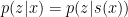
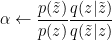
This is almost exactly rejection sampling. Remember that in general if you want to sample from 


Then, 

Why isn’t this exactly rejection sampling? In traditional descriptions of rejection sampling, you’d need to calculate 

Adding an 
To increase the chance of accepting (or make the algorithm work at all if 
Summary statistics
Another idea to reduce expense is to instead compare summary statistics. That is, find some function 


If we make this change, then the probability of returning 
![\displaystyle \begin{array}{rcl} \text{probability of returning }z^{*} & = & p(z^{*})\sum_{x}p(x\vert z^{*})I[s(x)=s(x^{*})].\\ & = & p(z^{*})p(s(x)\vert z^{*})\\ & = & p(s(x))p(z^{*}\vert s(x)). \end{array}](https://s0.wp.com/latex.php?latex=%5Cdisplaystyle++%5Cbegin%7Barray%7D%7Brcl%7D++%5Ctext%7Bprobability+of+returning+%7Dz%5E%7B%2A%7D+%26+%3D+%26+p%28z%5E%7B%2A%7D%29%5Csum_%7Bx%7Dp%28x%5Cvert+z%5E%7B%2A%7D%29I%5Bs%28x%29%3Ds%28x%5E%7B%2A%7D%29%5D.%5C%5C+%26+%3D+%26+p%28z%5E%7B%2A%7D%29p%28s%28x%29%5Cvert+z%5E%7B%2A%7D%29%5C%5C+%26+%3D+%26+p%28s%28x%29%29p%28z%5E%7B%2A%7D%5Cvert+s%28x%29%29.+%5Cend%7Barray%7D+&bg=ffffff&fg=000000&s=0&c=20201002)
Above we define ![{p(s'\vert z)=\sum_{x}p(x\vert z)I[s'=s(x)]}](https://s0.wp.com/latex.php?latex=%7Bp%28s%27%5Cvert+z%29%3D%5Csum_%7Bx%7Dp%28x%5Cvert+z%29I%5Bs%27%3Ds%28x%29%5D%7D&bg=ffffff&fg=000000&s=0&c=20201002)
![{p(s')=\sum_{x}p(x)I[s(x)=s'].}](https://s0.wp.com/latex.php?latex=%7Bp%28s%27%29%3D%5Csum_%7Bx%7Dp%28x%29I%5Bs%28x%29%3Ds%27%5D.%7D&bg=ffffff&fg=000000&s=0&c=20201002)
The probability of returning anything in a given round is

There’s good news and bad news about making this change.
Good news:
- We have improved the acceptance rate from
This could be much higher if there are many different datasets that yield the same summary statistics.
Bad news:
- This introduces errors in general. To avoid introducing error, we need that

Exponential family
Often, summary statistics are used even though they introduce errors. It seems to be a bit of a craft to find good summary statistics to speed things up without introducing too much error.
There is on appealing case where no error is introduced. Suppose 
Slop factors
If you’re using a slop factor, you can instead accept according to
This introduces the same kind of computation / accuracy tradeoff.

ABC-MCMC (Or likelihood-free MCMC)
Before getting to ABC-MCMC, suppose we just wanted for some reason to use Metropolis-Hastings to sample from the prior 

Algorithm: (Regular old Metropolis-Hastings)
- Initialize
- Repeat:
- Propose
from some proposal distribution
- Compute acceptance probability
.
- Generate
- If
then
.
- Propose

Now suppose we instead want to sample from the posterior 
Algorithm: (ABC-MCMC)
- Initialize
- Repeat:
- Propose
- Sample a synthetic dataset
.
- Compute acceptance probability
.
- Generate
- If
- Propose
There is only one difference: After proposing 
What this solves
There are two computational problems that the original ABC algorithm can encounter:
- The prior
may be a terrible proposal distribution for the posterior
- Even with a good proposal
The MCMC-ABC algorithm seems intended to deal with the first problem: If the proposal distributon 
On the other hand, MCMC-ABC algorithm seems to do little to address the second problem.
Justification
Now, why is this a correct algorithm? Consider the augmented distribution
![\displaystyle p(z,x^{*},x)=p(z,x^{*})I[x^{*}=x].](https://s0.wp.com/latex.php?latex=%5Cdisplaystyle++p%28z%2Cx%5E%7B%2A%7D%2Cx%29%3Dp%28z%2Cx%5E%7B%2A%7D%29I%5Bx%5E%7B%2A%7D%3Dx%5D.+&bg=ffffff&fg=000000&s=0&c=20201002)
We now want to sample from 

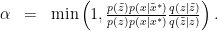
The acceptance probability will then be
![\displaystyle \begin{array}{rcl} \alpha & = & \min\left(1,\frac{p(\tilde{z},\tilde{x}^{*},x)}{p(z,x^{*},x)}\frac{q(z,x^{*}\vert\tilde{z},\tilde{x}^{*})}{q(\tilde{z},\tilde{x}^{*}\vert z,x^{*})}\right)\\ & = & \min\left(1,\frac{p(\tilde{z},\tilde{x}^{*})I[\tilde{x}^{*}=x]}{p(z,x^{*})I[x^{*}=x]}\frac{q(z\vert\tilde{z})p(x^{*}\vert z)}{q(\tilde{z}\vert z)p(\tilde{x}^{*}\vert\tilde{z})}\right) \end{array} .](https://s0.wp.com/latex.php?latex=%5Cdisplaystyle++%5Cbegin%7Barray%7D%7Brcl%7D++%5Calpha+%26+%3D+%26+%5Cmin%5Cleft%281%2C%5Cfrac%7Bp%28%5Ctilde%7Bz%7D%2C%5Ctilde%7Bx%7D%5E%7B%2A%7D%2Cx%29%7D%7Bp%28z%2Cx%5E%7B%2A%7D%2Cx%29%7D%5Cfrac%7Bq%28z%2Cx%5E%7B%2A%7D%5Cvert%5Ctilde%7Bz%7D%2C%5Ctilde%7Bx%7D%5E%7B%2A%7D%29%7D%7Bq%28%5Ctilde%7Bz%7D%2C%5Ctilde%7Bx%7D%5E%7B%2A%7D%5Cvert+z%2Cx%5E%7B%2A%7D%29%7D%5Cright%29%5C%5C+%26+%3D+%26+%5Cmin%5Cleft%281%2C%5Cfrac%7Bp%28%5Ctilde%7Bz%7D%2C%5Ctilde%7Bx%7D%5E%7B%2A%7D%29I%5B%5Ctilde%7Bx%7D%5E%7B%2A%7D%3Dx%5D%7D%7Bp%28z%2Cx%5E%7B%2A%7D%29I%5Bx%5E%7B%2A%7D%3Dx%5D%7D%5Cfrac%7Bq%28z%5Cvert%5Ctilde%7Bz%7D%29p%28x%5E%7B%2A%7D%5Cvert+z%29%7D%7Bq%28%5Ctilde%7Bz%7D%5Cvert+z%29p%28%5Ctilde%7Bx%7D%5E%7B%2A%7D%5Cvert%5Ctilde%7Bz%7D%29%7D%5Cright%29+%5Cend%7Barray%7D+.&bg=ffffff&fg=000000&s=0&c=20201002)
Since the original state 

![\displaystyle \begin{array}{rcl} \alpha & = & \min\left(1,\frac{p(\tilde{z})}{p(z)}\frac{q(z\vert\tilde{z})}{q(\tilde{z}\vert z)}\right)I[\tilde{x}^{*}=x]. \end{array}](https://s0.wp.com/latex.php?latex=%5Cdisplaystyle++%5Cbegin%7Barray%7D%7Brcl%7D++%5Calpha+%26+%3D+%26+%5Cmin%5Cleft%281%2C%5Cfrac%7Bp%28%5Ctilde%7Bz%7D%29%7D%7Bp%28z%29%7D%5Cfrac%7Bq%28z%5Cvert%5Ctilde%7Bz%7D%29%7D%7Bq%28%5Ctilde%7Bz%7D%5Cvert+z%29%7D%5Cright%29I%5B%5Ctilde%7Bx%7D%5E%7B%2A%7D%3Dx%5D.+%5Cend%7Barray%7D+&bg=ffffff&fg=000000&s=0&c=20201002)
Generalizations
If using summary statistics, you change ![{I[\tilde{x}^{*}=x]}](https://s0.wp.com/latex.php?latex=%7BI%5B%5Ctilde%7Bx%7D%5E%7B%2A%7D%3Dx%5D%7D&bg=ffffff&fg=000000&s=0&c=20201002)
![{I[s(\tilde{x}^{*})=s(x)].}](https://s0.wp.com/latex.php?latex=%7BI%5Bs%28%5Ctilde%7Bx%7D%5E%7B%2A%7D%29%3Ds%28x%29%5D.%7D&bg=ffffff&fg=000000&s=0&c=20201002)
More generally still, we could instead use the augmented distribution

The proposal 
Of course, this introduces some error.
Choosing
In practice, a good value of
(Thanks to Javier Burroni for helpful comments.)
]]>Some people feel intimidated by the prospect of putting a “theorem” into their papers. They feel that their results aren’t “deep” enough to justify this. Instead, they give the derivation and result inline as part of the normal text.
Sometimes that’s best. However, the purpose of a theorem is not to shout to the world that you’ve discovered something incredible. Rather, theorems are best thought of as an “API for ideas”. There are two basic purposes:
- To separate what you are claiming from your argument for that claim.
- To provide modularity to make it easier to understand or re-use your ideas.
To decide if you should create a theorem, ask if these goals will be advanced by doing so.
A thoughtful API makes software easier to use: The goal is to allow the user as much functionality as possible with as simple an interface as possible, while isolating implementation details. If you have a long chain a mathematical argument, you should choose what parts to write as theorems/lemmas in much the same way.
Many paper intermingle definitions, assumptions, proof arguments, and the final results. Have pity on the reader, and tell them in a single place what you are claiming, and under what assumptions. The “proof” section separates your evidence for your claim from the claim itself. Most readers want to understand your result before looking at the proof. Let them. Don’t make them hunt to figure out what your final result it.
Perhaps controversially, I suggest you should use the above reasoning even if you aren’t being fully mathematically rigorous. It’s still kinder to the reader to state your assumptions informally.
As an example of why it’s helpful to explicitly state your results, here’s an example from a seminal paper, so I’m sure the authors don’t mind. (Click on the image for a larger excerpt.)

This proof is well written. The problem is many small uncertainties that accumulate as you read it. If you try to understand exactly:
- What result is being stated?
- Under what assumptions does that result hold?
You will find that the proof “bleeds in” to the result itself. The convergence rate in 2.13 involves 
Of course, not every single claim needs to be written as a theorem/lemma/claim. If your result is simple to state and will only be used in a “one-off” manner, it may be clearer just to leave it in the text. That’s analogous to “inlining” a small function instead of creating another one.
2. Don’t fear the giant equation block.
I sometimes see a proof like this (for 
Take the quantity

Pulling out 

Factoring the denominator, this is

Etc.
For some proofs, the text between each line just isn’t that helpful. To a large degree it makes things more confusing– without an equality between the lines, you need to read the words to understand how each formula is supposed to be related to the previous one. Consider this alternative version of the proof:

In some cases, this reveals the overall structure of the proof better than a bunch of lines with interspersed text. If explanation is needed, it can be better to put it at the end, e.g. as “where line 2 follows from [blah] and line 3 follows from [blah]”.
It can also be helpful to put these explanations inline, i.e. to us a proof like

Again, this is not the best solution for all (or even most) cases, but I think it should be used more often than it is.
3. Use equivalence of inequalities when possible.
Many proofs involve manipulating chains of inequalities. When doing so, it should be obvious at what steps extra looseness may have been introduced. Suppose you have some positive constants 


People will often prove a result like the following:
Lemma: If 
Proof: Under the stated condition, we have that

That’s all correct, but doesn’t something feel slightly “magical” about the proof?
There are two problems: First, the proof reveals nothing anything about how you came up with the final answer. Second, the result leaves ambiguous if you have introduced additional looseness. Given the starting assumption, is it possible to prove a stronger bound?
I think the following lemma and proof are much better:
Lemma:
Proof: The following conditions are all equivalent:

The proof shows exactly how you arrived at the final result, and shows that there is no extra looseness. It’s better not to “pull a rabbit out of a hat” in a proof if not necessary.
This is arguably one of the most basic possible proof techniques, but is bizarrely underused. I think there’s two reasons why:
- Whatever need motivated the lemma is probably met by the first one above. The benefit of the second is mostly in providing more insight.
- Mathematical notation doesn’t encourage it. The sentence at the beginning of the proof is essential. If you see this merely as a series of inequalities, each implied by the one before, than it will not give the “only if” part of the result. You could conceivably try to write something like
, but this is awkward with multiple lines.

I use the (surprisingly controversial) convention of using a sans-serif font for random variables, rather than capital letters. I’m convinced this is the least-bad option for the machine learning literature, where many readers seem to find capital letter random variables distracting. It also allows you to distinguish matrix-valued random variables, though that isn’t used here.
]]>