Carview!

CARVIEW

MOTORHOMES

Select Language

HTTP/1.1 200 OK Date: Fri, 16 Jan 2026 02:40:43 GMT Server: Apache/2.4.65 (Debian) OpenSSL/1.1.1w mod_perl/2.0.11 Perl/v5.32.1 Last-Modified: Fri, 16 Jan 2026 00:00:19 GMT ETag: "2fe9d-6487606efa97b" Accept-Ranges: bytes Content-Length: 196253 Content-Type: application/atom+xml Tony Finch's blog Tony Finch dot@dotat.at https://dotat.at/ https://dotat.at/graphics/dotat-64.png https://dotat.at/@/blog.atom 2026-01-15T20:56:01Z GCRA vs leaky / token buckets https://dotat.at/@/2026-01-15-gcra.html 2026-01-15T20:23:39Z 2026-01-15T20:56:01Z In this note I’ll show why the rate limit algorithms GCRA, leaky bucket, and token bucket behave the same.

The parameters of the algorithms are a time window and a maximum quota of usage (e.g. requests or bytes) per window. The quota limits the size of a fast burst of requests. The maximum sustained rate is,

    rate = quota / window

Leaky bucket and token bucket store the time of the previous request, and a bucket counting the available capacity. The rate determines how quickly capacity becomes available.

It’s easy to see that leaky bucket and token bucket are equivalent, because they simply count in opposite directions:

    leaky -= (now - previous) * rate
    leaky = clamp(0, leaky, quota)
    leaky += cost
    previous = now
    return leaky < quota ? ALLOW : DENY
    tokens += (now - previous) * rate
    tokens = clamp(0, tokens, quota)
    tokens -= cost
    previous = now
    return tokens > 0 ? ALLOW : DENY

GCRA tracks a “not-before” time, and allows requests that occur after that point in time. The not-before time is normally in the recent past, and requests increase it towards and possibly (when the client is over its limit) beyond the present time.

    time = clamp(now - window, time, now)
    time += cost / rate
    return time < now ? ALLOW : DENY

It’s not trivially obvious that GCRA is equivalent to the other two. But we can convert the GCRA code into the leaky bucket code with a few transformations, as follows.

We can change from absolute time to relative time by taking now away from the equations:

    bucket = clamp(-window, time, 0)
    bucket += cost / rate
    return bucket < 0 ? ALLOW : DENY

But that change is incomplete: the stored bucket is relative to the time of the previous request. To make it relative to the current time, we need to remember when the previous request occurred, and after retrieving the bucket we need to shift it to account for the passage of time:

    bucket -= now - previous
    bucket = clamp(-window, time, 0)
    bucket += cost / rate
    previous = now
    return bucket < 0 ? ALLOW : DENY

Now we will change units to count tokens instead of seconds. We can do that by multiplying bucket by the rate, which is measured in tokens per second. Note that quota = window * rate.

    bucket -= (now - previous) * rate
    bucket = clamp(-quota, time, 0)
    bucket += cost
    previous = now
    return bucket < 0 ? ALLOW : DENY

Finally, add quota to bucket because positive numbers are nicer, and we end up with the leaky bucket code.

    bucket -= (now - previous) * rate
    bucket = clamp(0, time, quota)
    bucket += cost
    previous = now
    return bucket < quota ? ALLOW : DENY

Before writing this down I had a handwavey belief that these algoritms are equivalent – “it’s obvious!” enthusiatic gesturing. The tricky part was to explain the shift from relative to absolute time – why does GCRA use less storage? how does the passage of time become implicit? – so it was worth taking the time to make it as clear as I could.

The standard ITU GCRA variable names are:

Λ, the maximum rate, aka quota / window
T, the emission interval, 1 / Λ, aka window / quota
t_a, the arrival time, aka now
τ, the jitter tolerance; τ + T == quota
TAT, the theoretical arrival time

ITU GCRA compares TAT - τ < t_a where my GCRA compares time < now

My “not-before” time is roughly TAT - τ, but ITU GCRA does the clamp and increment in a different order, so the actual not-before time is TAT - τ - T. This corresponds to the difference between τ and quota.

]]> HTTP RateLimit headers https://dotat.at/@/2026-01-13-http-ratelimit.html 2026-01-14T02:34:22Z 2026-01-14T02:34:22Z There is an IETF draft that aims to standardize RateLimit header fields for HTTP. A RateLimit header in a successful response can inform a client when it might expect to be throttled, so it can avoid 429 Too Many Requests errors. Servers can also include RateLimit headers in a 429 response to make the error more informative.

The draft is in reasonably good shape. However as written it seems to require (or at least it assumes) that the server uses bad quota-reset rate limit algorithms. Quota-reset algorithms encourage clients into cyclic burst-pause behaviour; the draft has several paragraphs discussing this problem.

However, if we consider that RateLimit headers are supposed to tell the client what acceptable behaviour looks like, they can be used with any rate limit algorithm. (And it isn’t too hard to rephrase the draft so that it is written in terms of client behaviour instead of server behaviour.)

When a client has more work to do than will fit in a single window’s quota, linear rate limit algorithms such as GCRA encourage the client to smooth out its requests nicely. In this article I’ll describe how a server can use a linear rate limit algorithm with HTTP RateLimit headers.

spec summary
policy parameters
linear rate limit algorithm
other rate limiters

spec summary

The draft specifies two headers:

RateLimit-Policy: describes input parameters to a rate limit algorithm, which the server chooses based on the request in some unspecified way. The policies are expected to be largely static for a particular client. The parameters are,
- the name of the policy
- pk, the partition key
- q, the quota
- w, the window
- qu, the quota units
RateLimit: describes which policies the server applied to this request, and the output results of the rate limit algorithm. The results are likely to vary per request depending on client behaviour or server load, etc. The results are,
- the name of the policy
- pk, the partition key
- r, the available quota
- t, the effective window

Both headers can list multiple named policies.

To obey a policy, the client should not make more than q requests within w seconds. When it receives a response containing a RateLimit header, the client should not make more than r requests in the following t seconds.

(The draft calls r and t the “remaining quota” and “reset time”, which assumes too much about the rate limit algorithm. I prefer to describe them as the quota and window that are currently in effect.)

policy parameters

The client’s maximum sustained rate is

    rate = quota / window

On average the interval between requests at the maximum rate is

    interval = 1 / rate
             = window / quota

The draft establishes a standard collection of possible quota units, which determine how the cost of a request is counted.

qu="requests"
```
cost = 1
```
qu="content-bytes"
```
cost = size of content
```
qu="concurrent-requests"

(not applicable to this article)

The partition key pk identifies where the server keeps the per-client rate limit state. Typically a server will have a relatively small fixed set of rate limit policies, and a large dynamic collection of rate limit states.

linear rate limit algorithm

This linear rate limit algorithm is a variant of GCRA adapted to use HTTP RateLimit header terminology.

The per-client rate limit state is just a “not-before” timestamp. Requests are allowed if they occur after that point in time. The not-before timestamp is normally in the recent past, and requests increase it towards and possibly (when the client is over its limit) beyond the present time.

The output results contain r and t values for the RateLimit header. These must be whole numbers, though internally the algorithm needs subsecond precision because there can be many requests per second.

Get the client’s rate limit state. New clients are given a default not-before time in the distant past.
```
time = state[pk] or 0
```
Ensure the not-before time is within the sliding window. The minimum controls the client’s burst size quota; the maximum controls the penalty applied to abusive clients. This clamp() also protects against wild clock resets.
```
time = clamp(now - window, time, now)
```
Spend the nominal time consumed by the request.
```
time += interval * cost
```
The request is allowed if it occurs after the not-before time. The difference between the times determines the available quota and effective window. Round the quota down and the window up to whole numbers, so the client is given an underestimate of its service limit.
```
if now > time
    state[pk] = time
    d = now - time
    r = floor(d * rate)
    t = ceil(d)
    return ALLOW(r, t)
```
The request is denied if there is not enough time available. The available quota is zero, and the effective window is the not-before time, rounded up as before.
```
if time >= now
    r = 0
    t = ceil(time - now)
    return DENY(r, t)
```

That’s the core of the algorithm. There are a few refinements to consider, to do with strictness and cleanliness.

Over-limit clients can be treated more or less leniently:

The code above allows requests at the permitted rate regardless of how frequently the client makes attempts: denied requests are not counted.
Alternatively, the following code denies all requests from a client until its attempts slow down below the permitted rate. The cost is added to the effective window so that enough time is available when the client returns.
```
if time >= now
    state[pk] = time
    d = time - now
    d += interval * cost
    r = 0
    t = ceil(d)
    return ALLOW(r, t)
```
To apply an extra penalty time-out to clients that make requests within the not-before time, the server can increase the upper bound on the clamp() into the future.

Finally, it’s a good idea to have a background task that reclaims unnecessary state belonging to idle clients:

    for pk, time in state
        if time < now - window
            delete state[pk]

other rate limiters

The following discussion is mostly about explaining my claims in the introductory paragraphs at the start of this article.

There is a family of linear rate limit algorithms: GCRA behaves the same as a leaky bucket or a token bucket rate limiter (when they are implemented properly – there’s no need for a separate periodic leak / refill task), but GCRA uses less space per client (it doesn’t need an explicit bucket alongside the timestamp) and its code is simpler.

The HTTP RateLimit draft is based on algorithms that reset the quota and window at a predictable time regardless of client behaviour. (The draft allows other algorithms, but most of the text makes this assumption.) After a client makes a burst of requests, it has to wait until the reset time, then it is allowed to make another burst of requests.

Another class of algorithm is based on keeping a log of client activity within a sliding window in the recent past. (This is expensive and wasteful!) Sliding-window algorithms allow new requests when old requests age out, so they encourage clients to repeat past behaviour. If a client starts with a burst then it can burst again in each subsequent window.

By contrast, when a linear rate limiter allows a client to make a fast burst of requests, it shrinks the effective window and then keeps the effective window small while the client is busy.

Smaller quotas and windows restrict the burst size, so they require smoother behaviour than larger quotas and windows, even though the ratio quota / window describes the same maximum rate.

Automatically shrinking the effective window reduces the permitted burstiness of subsequent requests. As a result, linear rate limiters smooth out the interval between requests, as well as controlling the number of requests per window.

Other algorithms can make clients behave smoothly too.

A linear rate limiter indirectly assesses a client’s request rate by relating a request counter to the passage of time. By contrast, an exponential rate limiter directly measures a client’s average rate and allows or denies requests by comparing the rate to the limit.

An exponential rate limiter can be used with HTTP RateLimit headers in a similar manner to a linear rate limiter. That previous article explains how to calculate the effective window (called t_next) when a request is denied. When a request is allowed, the output results for a RateLimit header can be calculated as follows. (Beware, this snippet uses an awkward mixture of variable names from this article and the previous article.)

    if r_now < quota
        state[pk].time = t_now
        state[pk].rate = r_now
        a = quota - r_now
        r = floor(a)
        t = ceil(a * window / quota)
        return ALLOW(r, t)

The RateLimit header calculation for the exponential rate limiter is just the reciprocal of the linear rate limiter. It has the same smoothing effect for the same reasons.

I expect it’s possible to retrofit dynamic window shrinking on to other rate limit algorithms. But (as I wrote yesterday) it’s better to use a simple GCRA linear rate limiter.

PS. The terminology in this article is different from how I previously described rate limit algorithms: in the past I used rate = limit / period where the HTTP RateLimit draft uses quota / window.

]]> hybrid quota-linear rate limiter https://dotat.at/@/2026-01-12-hqlr.html 2026-01-13T00:12:01Z 2026-01-13T22:34:36Z A while back I wrote about the linear rate limit algorithms leaky bucket and GCRA. Since then I have been vexed by how common it is to implement rate limiting using complicated and wasteful algorithms (for example).

But linear (and exponential) rate limiters have a disadvantage: they can be slow to throttle clients whose request rate is above the limit but not super fast. And I just realised that this disadvantage can be unacceptable in some situations, when it’s imperative that no more than some quota of requests is accepted within a window of time.

In this article I’ll explore a way to enforce rate limit quotas more precisely, without undue storage costs, and without encouraging clients to oscillate between bursts and pauses. However I’m not sure it’s a good idea.

linear reaction time
fixed window quota resets
hybrid quota-linear algorithm
discussion
opinion

linear reaction time

How many requests does a linear rate limiter allow before throttling?

The parameters for a rate limiter are:

q, the permitted quota of requests
w, the accounting time window

So the maximum permitted rate is q/w.

Let’s consider a client whose rate is some multiple a > 1 of the permitted rate (a for abuse factor)

    c = a * q/w

I’ll model the rate limiter as a token bucket which starts off with q tokens at time 0. The bucket accumulates tokens at the permitted rate and the client consumes them at its request rate. (It is capped at q tokens but we can ignore that detail when a > 1.)

    b(t) = q + t*q/w - t*a*q/w

The time taken for n requests is

    t(n) = n/c = (n*w) / (a*q)

After n requests the bucket contains

    b(n) = q + n/a - n

The rate limter throttles the client when the bucket is empty.

    b(t) = 0 = q + t * (1 - a) * q/w
    0 = 1 - t * (a - 1) / w
    t = w / (a - 1)
    b(n) = 0 = q + n * (1/a - 1)
    0 = q - n * (a - 1) / a
    n = q * a / (a - 1)

For example, if the client is running at twice the permitted rate, a=2, they will be allowed q*2 requests within w seconds before they are throttled.

That’s a bit slow.

The problem is that the bucket starts with a full quota of tokens, and during the first window of time another quota-full is added. So a linear rate limiter seems to be more generous in its startup phase than its parameters suggest.

fixed window quota resets

This is a fairly common rate limit algorithm that enforces quotas more precisely than linear rate limiters. It is similar to a token bucket, but it resets the bucket to the full quota q after each window w.

The disadvantage of periodically resetting the bucket is that careless clients are likely to send a fast burst of requests every window. (A linear rate limiter will tend to smooth out requests from careless clients, though it can’t prevent deliberately abusive burstiness.) And a quota-reset rate limiter uses more space than a linear rate limiter: it needs a separate bucket counter as well as a timestamp.

each client has the time when its window started and a bucket of tokens

if c == NULL
    c = new Client
    c.bucket = quota
    c.time = now

reset the bucket when the window has expired

if c.time + window <= now
    c.bucket = quota
    c.time = now

the request is allowed if the client has a token to spend

if c.bucket >= 1
    c.bucket -= 1
    return ALLOW
else
    return DENY

hybrid quota-linear algorithm

The idea is to have two operating modes:

Low-traffic clients are allowed to make bursts of requests, because that’s good for interactive latency.
High-traffic clients are required to smooth out their requests to an even rate.

The algorithm switches to smooth mode when a client consumes its entire quota and the bucket reaches zero, and switches back to bursty mode when the bucket recovers to a full quota.

Bursty mode avoids being too generous by adding at most one quota of tokens to the bucket per window. Smooth mode also avoids being too generous by starting with an empty bucket.

I’ve written this pseudocode in a repetitive style because that makes each paragraph more independent of its context, though it is still somewhat stateful and the order of the clauses matters.

the rate limit is derived from the quota and window
```
rate = quota / window
```
a client that returns after a long absence is reinitialized like a new client; in bursty mode the time is the start of a fixed window and the bucket contains a whole number of tokens; we subtract one from the quota to account for the current request
```
fn reset()
    c.bucket = quota - 1
    c.time = now
    c.mode = BURSTY
    return ALLOW
```

initialize the state of a new client

if c == NULL
    c = new Client
    return reset()

reset the state when a bursty client’s window has expired

if c.mode == BURSTY
and c.time + window <= now
    return reset()

when a client consumes its last token, switch modes; in smooth mode the time is updated for every request and the bucket can hold fractional tokens; apply a negative penalty so we don’t allow any over-quota requests before the end of the fixed window; add one to allow the next request at the start of the next window
```
if c.mode == BURSTY
and c.bucket == 1
    remaining = c.time + window - now
    c.bucket = -remaining * rate + 1
    c.time = now
    c.mode = SMOOTH
    return ALLOW
```
smooth mode accumulates tokens proportional to the time since the client’s previous request; update the request time so that tokens accumulate at the same rate whether the request is allowed or denied
```
if c.mode == SMOOTH
    c.bucket += (now - c.time) * rate
    c.time = now
```

when the bucket has refilled, switch back to bursty mode

if c.mode == SMOOTH
and c.bucket >= quota
    return reset()

we have dealt with all the special cases; in either mode the request is allowed if the client has a token to spend
```
if c.bucket >= 1
    c.bucket -= 1
    return ALLOW
else
    return DENY
```

discussion

This hybrid algorithm has a similar effect to running both a quota-reset and a linear rate limiter in parallel, but it uses less space.

The precision of quota enforcement in smooth mode is maybe arguable: It guarantees that the client remains below the limit on average over the whole time it is in smooth mode. But if it slows down for a while (but not long enough to return to bursty mode) it can speed up again and make more requests than its quota within a window.

opinion

I think it’s a mistake to try to treat each time window in strict isolation when assessing a client’s request quota. A linear rate limiter only seems to be unduly generous on startup if you ignore the fact that the client was quiet in the previous window.

As well as being more expensive than necessary (in some cases disgracefully wasteful), algorithms like sliding-window and quota-reset encourage clients into cyclic burst-pause behaviour which is unhealthy for servers. And I’ve seen developers complaining about how annoying it is to use glut / famine rate limiters.

By contrast, rate limiters that measure longer-term average behaviour by keeping state across multiple windows can naturally encourage clients to smooth out their requests.

So on balance I think that instead of using this hybrid quota-linear rate limiter, you should reframe your problem so that you can use a simple linear rate limiter like GCRA.

]]> doubly dual shuffles https://dotat.at/@/2025-12-25-shuffle.html 2025-12-25T23:45:02Z 2025-12-25T23:45:02Z Here’s a pearlescent winter holiday gift for you!

There are four variants of the algorithm for shuffling an array, arising from two independent choices:

whether to swap elements in the higher or lower parts of the array
whether the boundary between the parts moves upwards or downwards

The variants are perfectly symmetrical, but they work in two fundamentally different ways: sampling or permutation.

The most common variant is Richard Durstenfeld’s shuffle algorithm, which moves the boundary downwards and swaps elements in the lower part of the array. Knuth describes it in TAOCP vol. 2 sect. 3.4.2; TAOCP doesn’t discuss the other variants.

(Obeying Stigler’s law, it is often called a “Fisher-Yates” shuffle, but their pre-computer algorithm is arguably different from the modern algorithm.)

the four variants

In the pseudocode below, min and max are the inclusive bounds on the array to be shuffled; the arguments to rand() are the inclusive bounds on its return value; and the loop bounds are inclusive too. I chose this style to make the symmetries more obvious.

In all variants, it’s possible for the indexes this (the boundary between the parts of the array) and that (chosen at random) to be the same, in which case the swap is a no-op.

I could have written the loop bounds as min and max instead of min+1 and max-1 to make the variants look as similar as possible, but it’s more realistic to omit the loop iterations when this and that are guaranteed to be equal.

It should be clear that rand() is invoked for spans of each size between 2 and N (where N = max - min + 1) so the algorithms produce N! possible permutations as expected.

boundary moves down, pick from lower

shuffle(a, min, max)
    for this = max to min+1 step -1
        that = rand(min, this)
        swap a[this] and a[that]

boundary moves up, pick from higher

shuffle(a, min, max)
    for this = min to max-1 step +1
        that = rand(this, max)
        swap a[this] and a[that]

boundary moves down, pick from higher

shuffle(a, min, max)
    for this = max-1 to min step -1
        that = rand(this, max)
        swap a[this] and a[that]

boundary moves up, pick from lower

shuffle(a, min, max)
    for this = min+1 to max step +1
        that = rand(min, this)
        swap a[this] and a[that]

the two kinds of shuffle

To merge four variants into two kinds, I’ll introduce some names that allow me to describe them independently of the direction of iteration. The todo part of the array is ahead of the iterator, i.e. lower if we are moving the boundary downwards, higher if we are moving it upwards. The done part of the array is behind the iterator, vice versa.

Earlier I called this the boundary between the parts, but that was a deliberate fencepost error which allowed me to gloss over an important difference. In fact the boundary is next to this, and which side it’s on depends on the kind of shuffle.

shuffle by sampling

The first two variants above work by sampling.

In this kind of shuffle, the indexes this and that are on the todo side of the boundary. We pick an element at random from the todo part of the array, and swap it into position next to the boundary. Then the boundary is moved so that the picked element is appended to the done part of the array.

The loop invariant or inductive hypothesis is that the done part of the array is a random sample of all the elements from the original array.

shuffle by permutation

The last two variants above work by permutation.

In this kind of shuffle, the indexes this and that are on the done side of the boundary. First we move the boundary to append an element from todo to done. Then we pick a random index in done, and swap the element next to the boundary into that position.

The loop invariant or inductive hypothesis is that the done part of the array is a random permutation of the elements that were originally in the same prefix or suffix of the array.

coda

I was inspired to write this by “The Fisher-Yates shuffle is backward” and the examples that were added to Wikipedia’s article on the Fisher-Yates shuffle a few months ago.

The article by “Possibly Wrong” correctly points out that there are two kinds of shuffle, but it misses out one of the four variants. Wikipedia’s examples show all four variants but they are cluttered by conventional array indexing, and it doesn’t explain there are actually two kinds of shuffle.

There’s a classic off-by-one mistake that turns a shuffle into Sattolo’s algorithm for cyclic permutations. It happens when the random bounds are too narrow, so that is never equal to this, and an element can never land in the same place that it started. This change has the same effect on both kinds of shuffle.

I enjoyed revisiting this old classic and trying to beautify it. I hope you like the results!

]]> how to draw a tetrapod https://dotat.at/@/2025-10-24-tetrapod.html 2025-10-24T21:40:51Z 2025-10-24T21:40:51Z Concrete tetrapods are used to dissipate wave energy in coastal defences.

There’s a bit of a craze for making tetrapod-shaped things: recently I’ve seen people making a plush tetrapod and a tetrapod lamp. So I thought it might be fun to model one.

I found a nice way to describe tetrapods that relies on very few arbitrary aesthetic choices.

Click here to play with an animated tetrapod which I made using three.js. (You can see its source code too.)

Click to skip to the recipe

a tetrapod constructed inside a cube, with lines marking the tetrahedron enclosed by the cube, and the circles used to construct the tetrapod

background and reference material

There is a patent for tetrapods written by the inventors of the tetrapod, Pierre Danel and Paul Anglès d’Auriac. It says,

The half angle a at the apex of the cone corresponding to one leg is between 9° and 14° while the leg length base width ratio b/c for each leg is between 0.85 and 1.15 and is preferably substantially 1/1.

One manufacturer has a diagram suggesting a taper of 10°.

A lot of pictures of tetrapods (one, two, three) have chunky chamfers at the ends of the legs. In some cases it looked to me like the angle of the chamfer matches the angle of the edges of the tetrahedron that the tetrapod is constructed from, which is the same as the angle of the faces of the cube that enclose the tetrahedron.

a surprising experiment

So I thought I would try constructing a tetrapod from the corners of a cube inwards.

My eyeball guesstimate sketch produced a result that’s amazingly neat. It’s the main reason I’m writing this blog post!

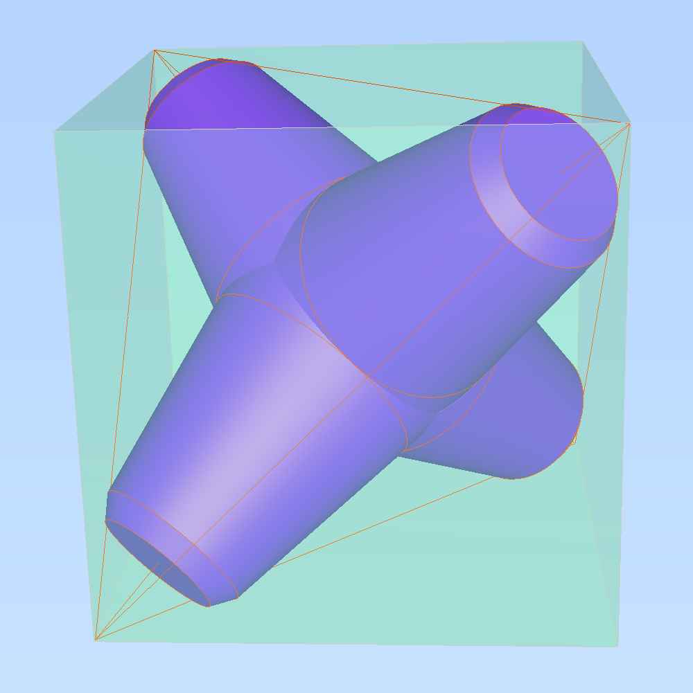
Using build123d and CQ-editor, I started with a cube centred on the origin enclosing a tetrahedron, with a common vertex at (100,100,100). I drew a pair of circles near the common vertex, just touching the faces of the cube and edges of the tetrahedron. These circles outlined where I thought the edges of the chamfer might be.

Using a taper angle of 10°, I found another circle centred on the origin that would be the base of the leg. I drew truncated cones to make the leg and chamfer, and replicated them to the three other axes of the tetrahedron.

With a bit of fettling of the sizes of the first two circles, I had a very plausible tetrapod!

To validate this sketch, I found the diameter of the circle around the leg near the centre of the cube where it just touches the x,y,z axes, and the distance from that circle to the end of the leg.

To my surprise, the width and length of the leg both came out very close to 100!

It’s good that they are about the same, because that’s what the inventors of the tetrapod specified. That means my eyeball guesstimate got the proportions about right. What’s amazing is that they match half the side length of the cube that I started with!

recipe for a tetrapod

You can read the source code for a tetrapod drawn using three.js and play with the resulting animation.

preliminaries

Pick a size.

The size is the length and diameter of each tetrapod leg, half the height of the tetrapod as it is constructed balancing on two legs, and a few percent less than half the height of the tetrapod when it’s standing on three legs.
The tetrapod is constructed inside a cube centred at the origin, with vertices at (± size, ± size, ± size). Inside the cube is a tetrahedron, and the tetrapod’s legs point towards its vertices.

In the picture above, the cube is shaded green, and the tetrahedron is outlined with straight red lines.
We will construct the positive leg along its main axis, the vector from the origin to the common vertex (+size, +size, +size).

The three other legs will be cloned from the positive leg.
The leg is constructed from truncated cones.

A cone is described by its taper, r / a = tan(θ), where a is the distance from the apex of the cone, and r is the radius of the circular section of the cone at that distance.

Every cone’s axis is the main axis, but their apex varies.
A cone is truncated by a circle with radius r and distance d from the origin along the main axis.

(Note that the apex distance a and origin distance d differ when the apex of the cone is not at the origin.)
We need two scaffolding cones.

The axis cone has its apex at the orign and its sides just touch the x,y,z axes.
```
axis_taper = sqrt(2)
```
derivation

z = (0,0,1)
xyz = (1,1,1)
z · xyz = |z| |xyz| cos(θ)
1 = 1 * sqrt(3) * cos(θ)
a / h = cos(θ) = sqrt(1/3)
r² = h² − a² = |z|² − a² = 1 − 1/3
tan(θ) = r / a = sqrt(2/3) / sqrt(1/3) = sqrt(2)

The face cone has its apex at the common vertex. Its sides just touch the faces of the cube along the same lines as the edges of the tetrahedron.
```
apex_d = size * sqrt(3)
face_taper = sqrt(1/2)
```
derivation

xy = (1,1,0)
xyz = (1,1,1)
xy · xyz = |xy| |xyz| cos(θ)
2 = sqrt(2) * sqrt(3) * cos(θ)
a / h = cos(θ) = sqrt(2/3)
r² = h² − a² = |xy|² − a² = 2 − 2*2/3
tan(θ) = r / a = sqrt(2/3) / sqrt(4/3) = sqrt(1/2)

circles

The leg is constructed from four circles: waist, thigh, ankle, sole. In the picture above, you can see the thigh, ankle, and sole circles outlined in red. The waist is hidden inside.

As required by the inventors of the tetrapod, our chosen size is equal to the diameter of the thigh, and to the distance between the thigh and the sole.

The thigh circles just touch each other at the x,y,z axes.

The foot of the tetrapod, between the ankle and the sole, is the chamfered part. It is a section of the face cone.

The ankle circle is chosen so that the taper of the main part of the leg is about 10°. It turns out that a nice round number, r = size / 3, makes the taper 10.41°.

To fill in the core of the tetrapod, between the thigh circles of the four legs, we will extrapolate the leg taper to find the waist circle whose centre is the origin.

Hence,

Locate the thigh circle from its radius in the axis cone
```
thigh_r = size / 2
thigh_d = 0 + thigh_r / axis_taper
```

Locate the ankle circle from its radius in the face cone

ankle_r = size / 3
ankle_d = apex_d - ankle_r / face_taper

The thigh circle and leg length determine the position of the sole circle, from which we get its radius
```
sole_d = thigh_d + size
sole_r = (apex_d - sole_d) * face_taper
```

The thigh and ankle give us the taper of the leg

leg_taper = (thigh_r - ankle_r)
          / (ankle_d - thigh_d)

Extrapolate back to the origin to find the radius of the waist
```
waist_d = 0
waist_r = thigh_r + thigh_d * leg_taper
```

legs

Make the positive leg from two truncated cones:

one between the waist and ankle,

one between the ankle and sole.
To make another leg, take a copy of the positive leg and rotate it 180° about the x or y or z axis.

Do this for all three axes to get all of the legs.

The legs overlap where their waists spread out around the origin. Conveniently, the legs meet at planes, so we can clip at these planes to make a model where they don’t overlap.

The positive leg meets the other legs at the three planes through the origin with normals:

    (1,1,0)
    (1,0,1)
    (0,1,1)

vital statistics

When standing on three legs with one leg vertical, this tetrapod is

2.09 * size tall
2.52 * size max wide
2.25 * size min wide

The radii of the key circles of the leg are

1/2 * size thigh
1/3 * size ankle
0.27 * size sole

The radii from the vertical axis to the ends of the base legs are

1.08 * size to point touching the ground
1.37 * size to furthest point

The taper of the leg is 10.4°.

The underside of the tetrapod is surprisingly close to flat.

0.17 * size between the ground and the cusp between the legs
9.0° angle between skin of legs and ground

The middle of each face of the tetrahedron is close to the core of the tetrapod. That’s partly because of the small 9° angle between the legs and the ground, which is parallel to a face of the tetrahedron. It’s also because the thigh circles protrude a tiny amount through each face, because they are slightly larger than the circles that just touch the x,y,z axes and the faces of the tetrahedron. These inner circles have a radius of sqrt(6/25) * size.

The cusp where three legs meet is slightly inside the face, by 0.015 * size.
The thigh circles are larger than the inner circles by 0.010 * size.

epilogue

It almost feels like the shape of the tetrapod was discovered rather than designed.

A tetrahedron nested in a cube is a fun framework for a shape. Using half the cube’s side length to determine the length and width of the legs seems like a natural choice. Maybe the choice was based on how close sqrt(6/25) and 1/2 are?

A third of the side length for the taper is a plausible option that turns out quite elegant. Maybe the chamfer at the foot is designed? I like the way it both hints at the cube from which it was constructed, and presumably has good engineering properties such as making the corner less prone to damage and easier to remove from its mould.

One thing I have not yet managed to work out (except by punting the problem to a CAD kernel) is exactly what ellipse is formed where the legs intersect. Investigations continue…

]]> a few notes on ratelimiting https://dotat.at/@/2025-09-14-ratelimit.html 2025-09-14T03:30:44Z 2025-09-14T03:30:44Z Last year I wrote a pair of articles about ratelimiting:

Recently, Chris “cks” Siebenmann has been working on ratelimiting HTTP bots that are hammering his blog. His articles prompted me to write some clarifications, plus a few practical anecdotes about ratelimiting email.

mea culpa

The main reason I wrote the GCRA article was to explain GCRA better without the standard obfuscatory terminology, and to compare GCRA with a non-stupid version of the leaky bucket algorithm. It wasn’t written with my old exponential ratelimiting in mind, so I didn’t match up the vocabulary.

In the exponential ratelimiting article I tried to explain how the different terms correspond to the same ideas, but I botched it by trying to be too abstract. So let’s try again.

parameters

It’s simplest to configure these ratelimiters (leaky bucket, GCRA, exponential) with two parameters:

limit
period

The maximum permitted average rate is calculated from these parameters by dividing them:

rate = limit / period

The period is the time over which client behaviour is averaged, which is also how long it takes for the ratelimiter to forget past behaviour. In my GCRA article I called it the window. Linear ratelimiters (leaky bucket and GCRA) are 100% forgetful after one period; the exponential ratelimiter is 67% forgetful.

The limit does double duty: as well as setting the maximum average rate (measured in requests per period) it sets the maximum size (measured in requests) of a fast burst of requests following a sufficiently long quiet gap.

how bursty

You can increase or decrease the burst limit – while keeping the average rate limit the same – by increasing or decreasing both the limit and the period.

For example, I might set limit = 600 requests per period = 1 hour. If I want to allow the same average rate, but with a smaller burst size, I might set limit = 10 requests per period = 1 minute.

anecdote

When I was looking after email servers, I set ratelimits for departmental mail servers to catch outgoing spam in case of compromised mail accounts or web servers. I sized these limits to a small multiple of the normal traffic so that legitimate mail was not delayed but spam could be stopped fairly quickly.

A typical setting was 200/hour, which is enough for a medium-sized department. (As a rule of thumb, expect people to send about 10 messages per day.)

An hourly limit is effective at catching problems quickly during typical working hours, but it can let out a lot of spam over a weekend.

So I would also set a second backstop limit like 1000/day, based on average daily traffic instead of peak hourly traffic. It’s a lower average rate that doesn’t forget bad behaviour so quickly, both of which help with weekend spam.

variable cost

Requests are not always fixed-cost. For example, you might want to count the request size in bytes when ratelimiting bandwidth.

The exponential algorithm calculates the instantaneous rate as

    r_inst = cost / interval

where cost is the size of the request and interval is the time since the previous request.

I’ve edited my GCRA algorithm to make the cost of requests more clear. In GCRA a request uses up some part of the client’s window, a nominal time measured in seconds. To convert a request’s size into time spent:

    spend = cost / rate

So the client’s earliest permitted time should be updated like:

    time += cost * period / limit

(In constrained implementations the period / limit factor can be precomputed.)

how lenient

When a client has used up its burst limit and is persistently making requests faster than its rate limit, the way the ratelimiter accepts or rejects requests is affected by the way it updates its memory of the client.

For exim’s ratelimit feature I provided two modes called “strict” and “leaky”. There is a third possibility: an intermediate mode which I will call “forgiving”.

The “leaky” mode is most lenient. An over-limit client will have occasional requests accepted at the maximum permitted rate. The rest of its requests will be rejected.

When a request is accepted, all of the client’s state is updated; when a request is rejected, the client’s state is left unchanged.

The lenient leaky mode works for both GCRA and exponential ratelimiting.
In “forgiving” mode, all of a client’s requests are rejected while it is over the ratelimit. As soon as it slows down below the ratelimit its requests will start being accepted.

When a request is accepted, all of the client’s state is updated; when a request is rejected, the client’s time is updated, but (in the exponential ratelimiter) not its measured rate.

The forgiving mode works for both GCRA and exponential ratelimiting.
In “strict” mode, all of a client’s requests are rejected while it is over the ratelimit, and requests continue to be rejected after a client has slowed down depending on how fast it previously was.

When a request is accepted or rejected, both of the client’s time and measured rate are updated.

The strict mode only works for exponential ratelimiting.

I only realised yesterday, from the discussion with cks, how a “forgiving” mode can be useful for the exponential ratelimiter, and how it corresponds to the less-lenient mode of linear leaky bucket and GCRA ratelimiters. (I didn’t describe the less-lenient mode in my GCRA article.)

anecdote

One of the hardest things about ratelimiting email was coming up with a policy that didn’t cause undue strife and unnecessary work.

When other mail servers (like the departmental server in the anecdote above) were sending mail through my relays, it made sense to use “leaky” ratelimiter mode with SMTP 450 temporary rejects. When there was a flood of mail, messages would be delayed and retried automatically.

When their queue size alerts went off, the department admin could take a look and respond as appropriate.

That policy worked fairly well.

However, when the sender was an end-user sending via my MUA message submission servers, they usually were not running software that could gracefully handle an SMTP 450 temporary rejection.

The most difficult cases were the various college and department alumni offices. Many of them would send out annual newsletters, using some dire combination of Microsoft Excel / Word / Outlook mailmerge, operated by someone with limited ability to repair a software failure.

In that situation, SMTP 450 errors broke their mailshots, causing enormous problems for the alumni office and their local IT support. (Not nice to realise I caused such trouble!)

The solution was to configure the ratelimiter in “strict” mode and “freeze” or quarantine over-limit bulk mail from MUAs. The “strict” mode ensured that everything after the initial burst of a spam run was frozen.

When the alert was triggered I inspected a sample of the frozen messages. If they were legitimate newsletters, I could thaw them for delivery and reset the user’s ratelimit. In almost all cases the user would not be disturbed.

If it turned out the user’s account was compromised and used to send spam, then I could get their IT support to help sort it out, and delete the frozen junk from the quarantine.

That policy worked OK: I was the only one who had to deal with my own false positives, and they were tolerably infrequent.

]]> first-class merges and cover letters https://dotat.at/@/2025-09-11-cover-letter.html 2025-09-11T01:26:47Z 2025-09-11T01:26:47Z Although it looks really good, I have not yet tried the Jujutsu (jj) version control system, mainly because it’s not yet clearly superior to Magit. But I have been following jj discussions with great interest.

One of the things that jj has not yet tackled is how to do better than git refs / branches / tags. As I underestand it, jj currently has something like Mercurial bookmarks, which are more like raw git ref plumbing than a high-level porcelain feature. In particular, jj lacks signed or annotated tags, and it doesn’t have branch names that always automatically refer to the tip.

This is clearly a temporary state of affairs because jj is still incomplete and under development and these gaps are going to be filled. But the discussions have led me to think about how git’s branches are unsatisfactory, and what could be done to improve them.

branch
merge
rebase
squash
fork
cover letters
previous branch
workflow
questions

branch

One of the huge improvements in git compared to Subversion was git’s support for merges. Subversion proudly advertised its support for lightweight branches, but a branch is not very useful if you can’t merge it: an un-mergeable branch is not a tool you can use to help with work-in-progress development.

The point of this anecdote is to illustrate that rather than trying to make branches better, we should try to make merges better and branches will get better as a consequence.

Let’s consider a few common workflows and how git makes them all unsatisfactory in various ways. Skip to cover letters and previous branch below where I eventually get to the point.

merge

A basic merge workflow is,

create a feature branch
hack, hack, review, hack, approve
merge back to the trunk

The main problem is when it comes to the merge, there may be conflicts due to concurrent work on the trunk.

Git encourages you to resolve conflicts while creating the merge commit, which tends to bypass the normal review process. Git also gives you an ugly useless canned commit message for merges, that hides what you did to resolve the conflicts.

If the feature branch is a linear record of the work then it can be cluttered with commits to address comments from reviewers and to fix mistakes. Some people like an accurate record of the history, but others prefer the repository to contain clean logical changes that will make sense in years to come, keeping the clutter in the code review system.

rebase

A rebase-oriented workflow deals with the problems of the merge workflow but introduces new problems.

Primarily, rebasing is intended to produce a tidy logical commit history. And when a feature branch is rebased onto the trunk before it is merged, a simple fast-forward check makes it trivial to verify that the merge will be clean (whether it uses separate merge commit or directly fast-forwards the trunk).

However, it’s hard to compare the state of the feature branch before and after the rebase. The current and previous tips of the branch (amongst other clutter) are recorded in the reflog of the person who did the rebase, but they can’t share their reflog. A force-push erases the previous branch from the server.

Git forges sometimes make it possible to compare a branch before and after a rebase, but it’s usually very inconvenient, which makes it hard to see if review comments have been addressed. And a reviewer can’t fetch past versions of the branch from the server to review them locally.

You can mitigate these problems by adding commits in --autosquash format, and delay rebasing until just before merge. However that reintroduces the problem of merge conflicts: if the autosquash doesn’t apply cleanly the branch should have another round of review to make sure the conflicts were resolved OK.

squash

When the trunk consists of a sequence of merge commits, the --first-parent log is very uninformative.

A common way to make the history of the trunk more informative, and deal with the problems of cluttered feature branches and poor rebase support, is to squash the feature branch into a single commit on the trunk instead of mergeing.

This encourages merge requests to be roughly the size of one commit, which is arguably a good thing. However, it can be uncomfortably confining for larger features, or cause extra busy-work co-ordinating changes across multiple merge requests.

And squashed feature branches have the same merge conflict problem as rebase --autosquash.

fork

Feature branches can’t always be short-lived. In the past I have maintained local hacks that were used in production but were not (not yet?) suitable to submit upstream.

I have tried keeping a stack of these local patches on a git branch that gets rebased onto each upstream release. With this setup the problem of reviewing successive versions of a merge request becomes the bigger problem of keeping track of how the stack of patches evolved over longer periods of time.

cover letters

Cover letters are common in the email patch workflow that predates git, and they are supported by git format-patch. Github and other forges have a webby version of the cover letter: the message that starts off a pull request or merge request.

In git, cover letters are second-class citizens: they aren’t stored in the repository. But many of the problems I outlined above have neat solutions if cover letters become first-class citizens, with a Jujutsu twist.

A first-class cover letter starts off as a prototype for a merge request, and becomes the eventual merge commit.

Instead of unhelpful auto-generated merge commits, you get helpful and informative messages. No extra work is needed since we’re already writing cover letters.

Good merge commit messages make good --first-parent logs.
The cover letter subject line works as a branch name. No more need to invent filename-compatible branch names!

Jujutsu doesn’t make you name branches, giving them random names instead. It shows the subject line of the topmost commit as a reminder of what the branch is for. If there’s an explicit cover letter the subject line will be a better summary of the branch as a whole.

I often find the last commit on a branch is some post-feature cleanup, and that kind of commit has a subject line that is never a good summary of its feature branch.
As a prototype for the merge commit, the cover letter can contain the resolution of all the merge conflicts in a way that can be shared and reviewed.

In Jujutsu, where conflicts are first class, the cover letter commit can contain unresolved conflicts: you don’t have to clean them up when creating the merge, you can leave that job until later.

If you can share a prototype of your merge commit, then it becomes possible for your collaborators to review any merge conflicts and how you resolved them.

To distinguish a cover letter from a merge commit object, a cover letter object has a “target” header which is a special kind of parent header. A cover letter also has a normal parent commit header that refers to earlier commits in the feature branch. The target is what will become the first parent of the eventual merge commit.

previous branch

The other ingredient is to add a “previous branch” header, another special kind of parent commit header. The previous branch header refers to an older version of the cover letter and, transitively, an older version of the whole feature branch.

Typically the previous branch header will match the last shared version of the branch, i.e. the commit hash of the server’s copy of the feature branch.

The previous branch header isn’t changed during normal work on the feature branch. As the branch is revised and rebased, the commit hash of the cover letter will change fairly frequently. These changes are recorded in git’s reflog or jj’s oplog, but not in the “previous branch” chain.

You can use the previous branch chain to examine diffs between versions of the feature branch as a whole. If commits have Gerrit-style or jj-style change-IDs then it’s fairly easy to find and compare previous versions of an individual commit.

The previous branch header supports interdiff code review, or allows you to retain past iterations of a patch series.

workflow

Here are some sketchy notes on how these features might work in practice.

One way to use cover letters is jj-style, where it’s convenient to edit commits that aren’t at the tip of a branch, and easy to reshuffle commits so that a branch has a deliberate narrative.

When you create a new feature branch, it starts off as an empty cover letter with both target and parent pointing at the same commit.
Alternatively, you might start a branch ad hoc, and later cap it with a cover letter.
If this is a small change and rebase + fast-forward is allowed, you can edit the “cover letter” to contain the whole change.
Otherwise, you can hack on the branch any which way. Shuffle the commits that should be part of the merge request so that they occur before the cover letter, and edit the cover letter to summarize the preceding commits.
When you first push the branch, there’s (still) no need to give it a name: the server can see that this is (probably) going to be a new merge request because the top commit has a target branch and its change-ID doesn’t match an existing merge request.
Also when you push, your client automatically creates a new instance of your cover letter, adding a “previous branch” header to indicate that the old version was shared. The commits on the branch that were pushed are now immutable; rebases and edits affect the new version of the branch.
During review there will typically be multiple iterations of the branch to address feedback. The chain of previous branch headers allows reviewers to see how commits were changed to address feedback, interdiff style.
The branch can be merged when the target header matches the current trunk and there are no conflicts left to resolve.

When the time comes to merge the branch, there are several options:

For a merge workflow, the cover letter is used to make a new commit on the trunk, changing the target header into the first parent commit, and dropping the previous branch header.
Or, if you like to preserve more history, the previous branch chain can be retained.
Or you can drop the cover letter and fast foward the branch on to the trunk.
Or you can squash the branch on to the trunk, using the cover letter as the commit message.

questions

This is a fairly rough idea: I’m sure that some of the details won’t work in practice without a lot of careful work on compatibility and deployability.

Do the new commit headers (“target” and “previous branch”) need to be headers?
What are the compatibility issues with adding new headers that refer to other commits?
How would a server handle a push of an unnamed branch? How could someone else pull a copy of it?
How feasible is it to use cover letter subject lines instead of branch names?
The previous branch header is doing a similar job to a remote tracking branch. Is there an opportunity to simplify how we keep a local cache of the server state?

Despite all that, I think something along these lines could make branches / reviews / reworks / merges less awkward. How you merge should me a matter of your project’s preferred style, without interference from technical limitations that force you to trade off one annoyance against another.

There remains a non-technical limitation: I have assumed that contributors are comfortable enough with version control to use a history-editing workflow effectively. I’ve lost all perspective on how hard this is for a newbie to learn; I expect (or hope?) jj makes it much easier than git rebase.

]]> strongly typed? https://dotat.at/@/2025-08-28-strongly-typed.html 2025-08-28T01:33:05Z 2025-08-28T01:33:05Z What does it mean when someone writes that a programming language is “strongly typed”?

I’ve known for many years that “strongly typed” is a poorly-defined term. Recently I was prompted on Lobsters to explain why it’s hard to understand what someone means when they use the phrase.

I came up with more than five meanings!

how strong?

The various meanings of “strongly typed” are not clearly yes-or-no. Some developers like to argue that these kinds of integrity checks must be completely perfect or else they are entirely worthless. Charitably (it took me a while to think of a polite way to phrase this), that betrays a lack of engineering maturity.

Software engineers, like any engineers, have to create working systems from imperfect materials. To do so, we must understand what guarantees we can rely on, where our mistakes can be caught early, where we need to establish processes to catch mistakes, how we can control the consequences of our mistakes, and how to remediate when somethng breaks because of a mistake that wasn’t caught.

strong how?

So, what are the ways that a programming language can be strongly or weakly typed? In what ways are real programming languages “mid”?

Statically typed as opposed to dynamically typed?

Many languages have a mixture of the two, such as run time polymorphism in OO languages (e.g. Java), or gradual type systems for dynamic languages (e.g. TypeScript).
Sound static type system?

It’s common for static type systems to be deliberately unsound, such as covariant subtyping in arrays or functions (Java, again). Gradual type systems migh have gaping holes for usability reasons (TypeScript, again).

And some type systems might be unsound due to bugs. (There are a few of these in Rust.)

Unsoundness isn’t a disaster, if a programmer won’t cause it without being aware of the risk.

For example: in Lean you can write “sorry” as a kind of “to do” annotation that deliberately breaks soundness; and Idris 2 has type-in-type so it accepts Girard’s paradox.
Type safe at run time?

Most languages have facilities for deliberately bypassing type safety, with an “unsafe” library module or “unsafe” language features, or things that are harder to spot. It can be more or less difficult to break type safety in ways that the programmer or language designer did not intend.

JavaScript and Lua are very safe, treating type safety failures as security vulnerabilities. Java and Rust have controlled unsafety. In C everything is unsafe.
Fewer weird implicit coercions?

There isn’t a total order here: for instance, C has implicit bool/int coercions, Rust does not; Rust has implicit deref, C does not.

There’s a huge range in how much coercions are a convenience or a source of bugs. For example, the PHP and JavaScript == operators are made entirely of WAT, but at least you can use === instead.
How fancy is the type system?

To what degree can you model properties of your program as types? Is it convenient to parse, not validate? Is the Curry-Howard correspondance something you can put into practice? Or is it only capable of describing the physical layout of data?

There are probably other meanings, e.g. I have seen “strongly typed” used to mean that runtime representations are abstract (you can’t see the underlying bytes); or in the past it sometimes meant a language with a heavy type annotation burden (as a mischaracterization of static type checking).

how to type

So, when you write (with your keyboard) the phrase “strongly typed”, delete it, and come up with a more precise description of what you really mean. The desiderata above are partly overlapping, sometimes partly orthogonal. Some of them you might care about, some of them not.

But please try to communicate where you draw the line and how fuzzy your line is.

]]> p-fast trie, but smaller https://dotat.at/@/2025-08-06-p-fast-trie.html 2025-08-06T17:19:09Z 2025-08-06T17:20:42Z Previously, I wrote some sketchy ideas for what I call a p-fast trie, which is basically a wide fan-out variant of an x-fast trie. It allows you to find the longest matching prefix or nearest predecessor or successor of a query string in a set of names in O(log k) cache misses, where k is the key length.

My initial sketch was more complicated and greedy for space than necessary, so here’s a simplified revision.

(“p” now stands for prefix.)

layout

A p-fast trie stores a lexicographically ordered set of names.

A name is a sequence of characters from some small-ish character set. For example, DNS names can be represented as a set of about 50 letters, digits, punctuation and escape characters, usually one per byte of name. Names that are arbitrary bit strings can be split into chunks of 6 bits to make a set of 64 characters.

Every unique prefix of every name is added to a hash table.

An entry in the hash table contains:

A shared reference to the closest name lexicographically greater than or equal to the prefix.

Multiple hash table entries will refer to the same name. A reference to a name might instead be a reference to a leaf object containing the name.
The length of the prefix.

To save space, each prefix is not stored separately, but implied by the combination of the closest name and prefix length.
A bitmap with one bit per possible character, corresponding to the next character after this prefix.

For every other prefix that matches this prefix and is one character longer than this prefix, a bit is set in the bitmap corresponding to the last character of the longer prefix.

search

The basic algorithm is a longest-prefix match.

Look up the query string in the hash table. If there’s a match, great, done.

Otherwise proceed by binary chop on the length of the query string.

If the prefix isn’t in the hash table, reduce the prefix length and search again. (If the empty prefix isn’t in the hash table then there are no names to find.)

If the prefix is in the hash table, check the next character of the query string in the bitmap. If its bit is set, increase the prefix length and search again.

Otherwise, this prefix is the answer.

predecessor

Instead of putting leaf objects in a linked list, we can use a more complicated search algorithm to find names lexicographically closest to the query string. It’s tricky because a longest-prefix match can land in the wrong branch of the implicit trie. Here’s an outline of a predecessor search; successor requires more thought.

During the binary chop, when we find a prefix in the hash table, compare the complete query string against the complete name that the hash table entry refers to (the closest name greater than or equal to the common prefix).

If the name is greater than the query string we’re in the wrong branch of the trie, so reduce the length of the prefix and search again.

Otherwise search the set bits in the bitmap for one corresponding to the greatest character less than the query string’s next character; if there is one remember it and the prefix length. This will be the top of the sub-trie containing the predecessor, unless we find a longer match.

If the next character’s bit is set in the bitmap, continue searching with a longer prefix, else stop.

When the binary chop has finished, we need to walk down the predecessor sub-trie to find its greatest leaf. This must be done one character at a time – there’s no shortcut.

thoughts

In my previous note I wondered how the number of search steps in a p-fast trie compares to a qp-trie.

I have some old numbers measuring the average depth of binary, 4-bit, 5-bit, 6-bit and 4-bit, 5-bit, dns qp-trie variants. A DNS-trie varies between 7 and 15 deep on average, depending on the data set. The number of steps for a search matches the depth for exact-match lookups, and is up to twice the depth for predecessor searches.

A p-fast trie is at most 9 hash table probes for DNS names, and unlikely to be more than 7. I didn’t record the average length of names in my benchmark data sets, but I guess they would be 8–32 characters, meaning 3–5 probes. Which is far fewer than a qp-trie, though I suspect a hash table probe takes more time than chasing a qp-trie pointer. (But this kind of guesstimate is notoriously likely to be wrong!)

However, a predecessor search might need 30 probes to walk down the p-fast trie, which I think suggests a linked list of leaf objects is a better option.

]]> p-fast trie: lexically ordered hash map https://dotat.at/@/2025-08-04-p-fast-trie.html 2025-08-04T20:52:21Z 2025-08-04T20:52:21Z Here’s a sketch of an idea that might or might not be a good idea. Dunno if it’s similar to something already described in the literature – if you know of something, please let me know via the links in the footer!

The gist is to throw away the tree and interior pointers from a qp-trie. Instead, the p-fast trie is stored using a hash map organized into stratified levels, where each level corresponds to a prefix of the key.

Exact-match lookups are normal O(1) hash map lookups. Predecessor / successor searches use binary chop on the length of the key. Where a qp-trie search is O(k), where k is the length of the key, a p-fast trie search is O(log k).

This smaller O(log k) bound is why I call it a “p-fast trie” by analogy with the x-fast trie, which has O(log log N) query time. (The “p” is for popcount.) I’m not sure if this asymptotic improvement is likely to be effective in practice; see my thoughts towards the end of this note.

layout

A p-fast trie consists of:

Leaf objects, each of which has a name.

Each leaf object refers to its successor forming a circular linked list. (The last leaf refers to the first.)

Multiple interior nodes refer to each leaf object.
A hash map containing every (strict) prefix of every name in the trie. Each prefix maps to a unique interior node.

Names are treated as bit strings split into chunks of (say) 6 bits, and prefixes are whole numbers of chunks.
An interior node contains a (1<<6) == 64 wide bitmap with a bit set for each chunk where prefix+chunk matches a key.

Following the bitmap is a popcount-compressed array of references to the leaf objects that are the closest predecessor of the corresponding prefix+chunk key.

Prefixes are strictly shorter than names so that we can avoid having to represent non-values after the end of a name, and so that it’s OK if one name is a prefix of another.

The size of chunks and bitmaps might change; 6 is a guess that I expect will work OK. For restricted alphabets you can use something like my DNS trie name preparation trick to squash 8-bit chunks into sub-64-wide bitmaps.

In Rust where cross-references are problematic, there might have to be a hash map that owns the leaf objects, so that the p-fast trie can refer to them by name. Or use a pool allocator and refer to leaf objects by numerical index.

search

To search, start by splitting the query string at its end into prefix + final chunk of bits. Look up the prefix in the hash map and check the chunk’s bit in the bitmap. If it’s set, you can return the corresponding leaf object because it’s either an exact match or the nearest predecessor.

If it isn’t found, and you want the predecessor or successor, continue with a binary chop on the length of the query string.

Look up the chopped prefix in the hash map. The next chunk is the chunk of bits in the query string immediately after the prefix.

If the prefix is present and the next chunk’s bit is set, remember the chunk’s leaf pointer, make the prefix longer, and try again.

If the prefix is present and the next chunk’s bit is not set and there’s a lesser bit that is set, return the leaf pointer for the lesser bit. Otherwise make the prefix shorter and try again.

If the prefix isn’t present, make the prefix shorter and try again.

When the binary chop bottoms out, return the longest-matching leaf you remembered.

The leaf’s key and successor bracket the query string.

modify

When inserting a name, all its prefixes must be added to the hash map from longest to shortest. At the point where it finds that the prefix already exists, the insertion routine needs to walk down the (implicit) tree of successor keys, updating pointers that refer to the new leaf’s predecessor so they refer to the new leaf instead.

Similarly, when deleting a name, remove every prefix from longest to shortest from the hash map where they only refer to this leaf. At the point where the prefix has sibling nodes, walk down the (implicit) tree of successor keys, updating pointers that refer to the deleted leaf so they refer to its predecessor instead.

I can’t “just” use a concurrent hash map and expect these algorithms to be thread-safe, because they require multiple changes to the hashmaps. I wonder if the search routine can detect when the hash map is modified underneath it and retry.

thoughts

It isn’t obvious how a p-fast trie might compare to a qp-trie in practice.

A p-fast trie will use a lot more memory than a qp-trie because it requires far more interior nodes. They need to exist so that the random-access binary chop knows whether to shorten or lengthen the prefix.

To avoid wasting space the hash map keys should refer to names in leaf objects, instead of making lots of copies. This is probably tricky to get right.

In a qp-trie the costly part of the lookup is less than O(k) because non-branching interior nodes are omitted. How does that compare to a p-fast trie’s O(log k)?

Exact matches in a p-fast trie are just a hash map lookup. If they are worth optimizing then a qp-trie could also be augmented with a hash map.

Many steps of a qp-trie search are checking short prefixes of the key near the root of the tree, which should be well cached. By contrast, a p-fast trie search will typically skip short prefixes and instead bounce around longer prefixes, which suggests its cache behaviour won’t be so friendly.

A qp-trie predecessor/successor search requires two traversals, one to find the common prefix of the key and another to find the prefix’s predecessor/successor. A p-fast trie requires only one.

]]> clamp / median / range https://dotat.at/@/2025-07-02-cmp.html 2025-07-02T01:33:08Z 2025-07-02T01:33:08Z Here are a few tangentially-related ideas vaguely near the theme of comparison operators.

comparison style
clamp style
clamp is median
clamp in range
range style
style clash?

comparison style

Some languages such as BCPL, Icon, Python have chained comparison operators, like

    if min <= x <= max:
        ...

In languages without chained comparison, I like to write comparisons as if they were chained, like,

    if min <= x && x <= max {
        // ...
    }

A rule of thumb is to prefer less than (or equal) operators and avoid greater than. In a sequence of comparisons, order values from (expected) least to greatest.

clamp style

The clamp() function ensures a value is between some min and max,

    def clamp(min, x, max):
        if x < min: return min
        if max < x: return max
        return x

I like to order its arguments matching the expected order of the values, following my rule of thumb for comparisons – and the description of what clamp() does. (I used this flavour of clamp() in my article about GCRA.) But I seem to be unusual in this preference, based on a few examples I have seen recently.

clamp is median

Last month, Fabian Giesen pointed out a way to resolve this difference of opinion: A function that returns the median of three values is equivalent to a clamp() function that doesn’t care about the order of its arguments.

This version is written so that it returns NaN if any of its arguments is NaN. (When an argument is NaN, both of its comparisons will be false.)

    fn med3(a: f64, b: f64, c: f64) -> f64 {
        match (a <= b, b <= c, c <= a) {
            (false, false, false) => f64::NAN,
            (false, false, true)  => b, //  a > b > c
            (false, true,  false) => a, //  c > a > b
            (false, true,  true)  => c, // b <= c <= a
            (true,  false, false) => c, //  b > c > a
            (true,  false, true)  => a, // c <= a <= b
            (true,  true,  false) => b, // a <= b <= c
            (true,  true,  true)  => b, // a == b == c
        }
    }

When two of its arguments are constant, med3() should compile to the same code as a simple clamp(); but med3()’s misuse-resistance comes at a small cost when the arguments are not known at compile time.

clamp in range

If your language has proper range types, there is a nicer way to make clamp() resistant to misuse:

    fn clamp(x: f64, r: RangeInclusive<f64>) -> f64 {
        let (&min,&max) = (r.start(), r.end());
        if x < min { return min }
        if max < x { return max }
        return x;
    }
    let x = clamp(x, MIN..=MAX);

range style

For a long time I have been fond of the idea of a simple counting for loop that matches the syntax of chained comparisons, like

    for min <= x <= max:
        ...

By itself this is silly: too cute and too ad-hoc.

I’m also dissatisfied with the range or slice syntax in basically every programming language I’ve seen. I thought it might be nice if the cute comparison and iteration syntaxes were aspects of a more generally useful range syntax, but I couldn’t make it work.

Until recently when I realised I could make use of prefix or mixfix syntax, instead of confining myself to infix.

So now my fantasy pet range syntax looks like

    >= min < max    // half-open
    >= min <= max   // inclusive

And you might use it in a pattern match

    if x is >= min < max {
        // ...
    }

Or as an iterator

    for x in >= min < max {
        // ...
    }

Or to take a slice

    xs[>= min < max]

style clash?

It’s kind of ironic that these range examples don’t follow the left-to-right, lesser-to-greater rule of thumb that this post started off with. (x is not lexically between min and max!)

But that rule of thumb is really intended for languages such as C that don’t have ranges. Careful stylistic conventions can help to avoid mistakes in nontrivial conditional expressions.

It’s much better if language and library features reduce the need for nontrivial conditions and catch mistakes automatically.

]]> Golang and Let's Encrypt: a free software story https://dotat.at/@/2025-06-28-boulder.html 2025-06-26T01:41:49Z 2025-06-26T01:50:23Z Here’s a story from nearly 10 years ago.

the bug

I think it was my friend Richard Kettlewell who told me about a bug he encountered with Let’s Encrypt in its early days in autumn 2015: it was failing to validate mail domains correctly.

the context

At the time I had previously been responsible for Cambridge University’s email anti-spam system for about 10 years, and in 2014 I had been given responsibility for Cambridge University’s DNS. So I knew how Let’s Encrypt should validate mail domains.

Let’s Encrypt was about one year old. Unusually, the code that runs their operations, Boulder, is free software and open to external contributors.

Boulder is written in Golang, and I had not previously written any code in Golang. But its reputation is to be easy to get to grips with.

So, in principle, the bug was straightforward for me to fix. How difficult would it be as a Golang newbie? And what would Let’s Encrypt’s contribution process be like?

the hack

I cloned the Boulder repository and had a look around the code.

As is pretty typical, there are a couple of stages to fixing a bug in an unfamiliar codebase:

work out where the problem is
try to understand if the obvious fix could be better

In this case, I remember discovering a relatively substantial TODO item that intersected with the bug. I can’t remember the details, but I think there were wider issues with DNS lookups in Boulder. I decided it made sense to fix the immediate problem without getting involved in things that would require discussion with Let’s Encrypt staff.

I faffed around with the code and pushed something that looked like it might work.

A fun thing about this hack is that I never got a working Boulder test setup on my workstation (or even Golang, I think!) – I just relied on the Let’s Encrypt cloud test setup. The feedback time was very slow, but it was tolerable for a simple one-off change.

the fix

My pull request was small, +48-14.

After a couple of rounds of review and within a few days, it was merged and put into production!

A pleasing result.

the upshot

I thought Golang (at least as it was used in the Boulder codebase) was as easy to get to grips with as promised. I did not touch it again until several years later, because there was no need to, but it seemed fine.

I was very impressed by the Let’s Encrypt continuous integration and automated testing setup, and by their low-friction workflow for external contributors. One of my fastest drive-by patches to get into worldwide production.

My fix was always going to be temporary, and all trace of it was overwritten years ago. It’s good when “temporary” turns out to be true!

the point

I was reminded of this story in the pub this evening, and I thought it was worth writing down. It demonstrated to me that Let’s Encrypt really were doing all the good stuff they said they were doing.

So thank you to Let’s Encrypt for providing an exemplary service and for giving me a happy little anecdote.

]]> performance of random floats https://dotat.at/@/2025-06-08-floats.html 2025-06-08T02:08:35Z 2025-06-09T16:50:27Z A couple of years ago I wrote about random floating point numbers. In that article I was mainly concerned about how neat the code is, and I didn’t pay attention to its performance.

Recently, a comment from Oliver Hunt and a blog post from Alisa Sireneva prompted me to wonder if I made an unwarranted assumption. So I wrote a little benchmark, which you can find in pcg-dxsm.git.

(Note 2025-06-09: I’ve edited this post substantially after discovering some problems with the results.)

recap
code
- bithack
- multiply
benchmark
results
conclusion

recap

Briefly, there are two basic ways to convert a random integer to a floating point number between 0.0 and 1.0:

Use bit fiddling to construct an integer whose format matches a float between 1.0 and 2.0; this is the same span as the result but with a simpler exponent. Bitcast the integer to a float and subtract 1.0 to get the result.
Shift the integer down to the same range as the mantissa, convert to float, then multiply by a scaling factor that reduces it to the desired range. This produces one more bit of randomness than the bithacking conversion.

(There are other less basic ways.)

code

The double precision code for the two kinds of conversion is below. (Single precision is very similar so I’ll leave it out.)

It’s mostly as I expect, but there are a couple of ARM instructions that surprised me.

bithack

The bithack function looks like:

    double bithack52(uint64_t u) {
        u = ((uint64_t)(1023) << 52) | (u >> 12);
        return(bitcast(double, u) - 1.0);
    }

It translates fairly directly to amd64 like this:

    bithack52:
        shr     rdi, 12
        movabs  rax, 0x3ff0000000000000
        or      rax, rdi
        movq    xmm0, rax
        addsd   xmm0, qword ptr [rip + .number]
        ret
    .number:
        .quad   0xbff0000000000000

On arm64 the shift-and-or becomes one bfxil instruction (which is a kind of bitfield move), and the constant -1.0 is encoded more briefly. Very neat!

    bithack52:
        mov     x8, #0x3ff0000000000000
        fmov    d0, #-1.00000000
        bfxil   x8, x0, #12, #52
        fmov    d1, x8
        fadd    d0, d1, d0
        ret

multiply

The shift-convert-multiply function looks like this:

    double multiply53(uint64_t u) {
        return ((double)(u >> 11) * 0x1.0p-53);
    }

It translates directly to amd64 like this:

    multiply53:
        shr       rdi, 11
        cvtsi2sd  xmm0, rdi
        mulsd     xmm0, qword ptr [rip + .number]
        ret
    .number:
        .quad     0x3ca0000000000000

GCC and earlier versions of Clang produce the following arm64 code, which is similar though it requires more faff to get the constant into the right register.

    multiply53:
        lsr     x8, x0, #11
        mov     x9, #0x3ca0000000000000
        ucvtf   d0, x8
        fmov    d1, x9
        fmul    d0, d0, d1
        ret

Recent versions of Clang produce this astonishingly brief two instruction translation: apparently you can convert fixed-point to floating point in one instruction, which gives us the power of two scale factor for free!

    multiply53:
        lsr     x8, x0, #11
        ucvtf   d0, x8, #53
        ret

benchmark

My benchmark has 2 x 2 x 2 tests:

bithacking vs multiplying
32 bit vs 64 bit
sequential integers vs random integers

I ran the benchmark on my Apple M1 Pro and my AMD Ryzen 7950X.

These functions are very small and work entirely in registers so it has been tricky to measure them properly.

To prevent the compiler from inlining and optimizing the benchmark loop to nothing, the functions are compiled in a separate translation unit from the test harness. This is not enough to get plausible measurements because the CPU overlaps successive iterations of the loop, so we also use fence instructions.

On arm64, a single ISB (instruction stream barrier) in the loop is enough to get reasonable measurements.

I have not found an equivalent of ISB on amd64, so I’m using MFENCE. It isn’t effective unless I pass the argument and return values via pointers (because it’s a memory fence) and place MFENCE instructions just before reading the argument and just after writing the result.

results

In the table below, the leftmost column is the number of random bits; “old” is arm64 with older clang, “arm” is newer clang, “amd” is gcc.

The first line is a baseline do-nothing function, showing the overheads of the benchmark loop, function call, load argument, store return, and fences.

The upper half measures sequential numbers, the bottom half is random numbers. The times are nanoseconds per operation.

         old    arm    amd
    00  21.44  21.41  21.42
    23  24.28  24.31  22.19
    24  25.24  24.31  22.94
    52  24.31  24.28  21.98
    53  25.32  24.35  22.25
    23  25.59  25.56  22.86
    24  26.55  25.55  23.03
    52  27.83  27.81  23.93
    53  28.57  27.84  25.01

The times vary a little from run to run but the difference in speed of the various loops is reasonably consistent.

The numbers on arm64 are reasonably plausible. The most notable thing is that the “old” multiply conversion is about 3 or 4 clock cycles slower, but with a newer compiler that can eliminate the multiply, it’s the same speed as the bithacking conversion.

On amd64 the multiply conversion is about 1 or 2 clock cycles slower than the bithacking conversion.

conclusion

The folklore says that bithacking floats is faster than normal integer to float conversion, and my results generally agree with that, apart from on arm64 with a good compiler. It would be interesting to compare other CPUs to get a better idea of when the folklore is right or wrong – or if any CPUs perform the other way round!

]]> moka pot notes https://dotat.at/@/2025-06-01-bialetti.html 2025-06-01T15:56:02Z 2025-06-01T15:56:02Z In hot weather I like to drink my coffee in an iced latte. To make it, I have a very large Bialetti Moka Express. Recently when I got it going again after a winter of disuse, it took me a couple of attempts to get the technique right, so here are some notes as a reminder to my future self next year.

It’s worth noting that I’m not fussy about my coffee: I usually drink pre-ground beans from the supermarket, with cream (in winter hot coffee) or milk and ice.

basic principle

When I was getting the hang of my moka pot, I learned from YouTube coffee geeks such as James Hoffmann that the main aim is for the water to be pushed through the coffee smoothly and gently. Better to err on the side of too little flow than too much.

I have not had much success trying to make fine temperature adjustments while the coffee is brewing, because the big moka pot has a lot of thermal inertia: it takes a long time for any change in gas level to have any effect on on the coffee flow.

routine

fill the kettle and turn it on
put the moka pot’s basket in a mug to keep it stable
fill it with coffee (mine needs about 4 Aeropress scoops)
tamp it down firmly [1]
when the kettle has boiled, fill the base of the pot to just below the pressure valve (which is also just below the filter screen in the basket)
insert the coffee basket, making sure there are no stray grounds around the edge where the seal will mate
screw on the upper chamber firmly
put it on a small gas ring turned up to the max [2]
leave the lid open and wait for the coffee to emerge
immediately turn the gas down to the minimum [3]
the coffee should now come out in a steady thin stream without spluttering or stalling
when the upper chamber is filled near the mouths of the central spout, it’ll start fizzing or spluttering [4]
turn off the gas and pour the coffee into a carafe

notes

If I don’t tamp the grounds, the pot tends to splutter. I guess tamping gives the puck better integrity to resist channelling, and to keep the water under even pressure. Might be an effect of the relatively coarse supermarket grind?
It takes a long time to get the pot back up to boiling point and I’m not sure that heating it up slower helps. The main risk, I think, is overshooting the ideal steady brewing state too much, but:
With my moka pot on my hob the lowest gas flow on the smallest rings is just enough to keep the coffee flowing without stalling. The flow when the coffee first emerges is relatively fast, and it slows to the steady state several seconds after I turn the heat down, so I think the overshoot isn’t too bad.
This routine turns almost all of the water into coffee, which Hoffmann suggests is a good result, and a sign that the pressure and temperature aren’t getting too high.

]]> the algebra of dependent types https://dotat.at/@/2025-05-28-types.html 2025-05-29T00:07:51Z 2025-05-29T00:26:38Z TIL (or this week-ish I learned) why big-sigma and big-pi turn up in the notation of dependent type theory.

I’ve long been aware of the zoo of more obscure Greek letters that turn up in papers about type system features of functional programming languages, μ, Λ, Π, Σ. Their meaning is usually clear from context but the reason for the choice of notation is usually not explained.

I recently stumbled on an explanation for Π (dependent functions) and Σ (dependent pairs) which turn out to be nicer than I expected, and closely related to every-day algebraic data types.

sizes of types

The easiest way to understand algebraic data types is by counting the inhabitants of a type. For example:

the unit type () has one inhabitant, (), and the number 1 is why it’s called the unit type;
the bool type hass two inhabitants, false and true.

I have even seen these types called 1 and 2 (cruelly, without explanation) in occasional papers.

product types

Or pairs or (more generally) tuples or records. Usually written,

    (A, B)

The pair contains an A and a B, so the number of possible values is the number of possible A values multiplied by the number of possible B values.

So it is spelled in type theory (and in Standard ML) like,

    A * B

sum types

Or disjoint union, or variant record. Declared in Haskell like,

        data Either a b
            = Left a
            | Right b

Or in Rust like,

        enum Either<A, B> {
            Left(A),
            Right(B),
        }

A value of the type is either an A or a B, so the number of possible values is the number of A values plus the number of B values.

So it is spelled in type theory like,

    A + B

dependent pairs

In a dependent pair, the type of the second element depends on the value of the first. The classic example is a slice, roughly,

        struct IntSlice {
            len: usize,
            elem: &[i64; len],
        }

(This might look a bit circular, but the idea is that an array [i64; N] must be told how big it is – its size is an explicit part of its type – but an IntSlice knows its own size. The traditional dependent “vector” type is a sized linked list, more like my array type than my slice type.)

The classic way to write a dependent pair in type theory is like,

Σ len: usize . Array(Int, len)

The big sigma binds a variable that has a type annotation, with a scope covering the expression after the dot – similar syntax to a typed lambda expression.

We can expand a simple example like this into a many-armed sum type: either an array of length zero, or an array of length 1, or an array of length 2, … but in a sigma type the discriminant is user-defined instead of hidden.

The number of possible values of the type comes from adding up all the alternatives, a summation just like the big sigma summation we were taught in school.

\sum_{a \in A} B_{a}

When the second element doesn’t depend on the first element, we can count the inhabitants like,

\sum_{A} B = A * B

And the sigma type simplifies to a product type.

telescopes

An aside from the main topic of these notes, I also recently encountered the name “telescope” for a multi-part dependent tuple or record.

The name “telescope” comes from de Bruijn’s AUTOMATH, one of the first computerized proof assistants. (I first encountered de Bruijn as the inventor of numbered lambda bindings.)

dependent functions

The return type of a dependent function can vary according to the argument it is passed.

For example, to construct an array we might write something like,

        fn repeat_zero(len: usize) -> [i64; len] {
            [0; len]
        }

The classic way to write the type of repeat_zero() is very similar to the IntSlice dependent pair, but with a big pi instead of a big sigma:

Π len: usize . Array(Int, len)

Mmm, pie.

To count the number of possible (pure, total) functions A ➞ B, we can think of each function as a big lookup table with A entries each containing a B. That is, a big tuple (B, B, … B), that is, B * B * … * B, that is, B^A. Functions are exponential types.

We can count a dependent function, where the number of possible Bs depends on which A we are passed,

\prod_{a \in A} B_{a}

danger

I have avoided the terms “dependent sum” and “dependent product”, because they seem perfectly designed to cause confusion over whether I am talking about variants, records, or functions.

It kind of makes me want to avoid algebraic data type jargon, except that there isn’t a good alternative for “sum type”. Hmf.

]]> the penultimate conditional syntax https://dotat.at/@/2025-05-13-if-is.html 2025-05-13T21:49:41Z 2025-05-13T21:49:41Z About half a year ago I encountered a paper bombastically titled “the ultimate conditional syntax”. It has the attractive goal of unifying pattern match with boolean if tests, and its solution is in some ways very nice. But it seems over-complicated to me, especially for something that’s a basic work-horse of programming.

I couldn’t immediately see how to cut it down to manageable proportions, but after reading syntactic musings on match expressions by Yoshua Wuyts a couple of weeks ago, I had an idea. I’ll outline it under the “penultimate conditionals” heading below, after reviewing the UCS and explaining my motivation.

what the UCS?
whence UCS
out of scope
penultimate conditionals
dangling syntax
examples
antepenultimate breath

what the UCS?

The ultimate conditional syntax does several things which are somewhat intertwined and support each other.

An “expression is pattern” operator allows you to do pattern matching inside boolean expressions.

Like “match” but unlike most other expressions, “is” binds variables whose scope is the rest of the boolean expression that might be evaluated when the “is” is true, and the consequent “then” clause.
You can “split” tests to avoid repeating parts that are the same in successive branches. For example,
```
    if num < 0 then -1 else
    if num > 0 then +1 else 0
```
can be written
```
    if num < 0 then -1
           > 0 then +1
               else  0
```
The example shows a split before an operator, where the left hand operand is the same and the rest of the expression varies. You can split after the operator when the operator is the same, which is common for “is” pattern match clauses.
Indentation-based syntax (an offside rule) reduces the amount of punctuation that splits would otherwise need. An explicit version of the example above is
```
    if { x { { < { 0 then −1 } };
             { > { 0 then +1 } }; else 0 } }
```
(This example is written in the paper on one line. I’ve split it for narrow screens, which exposes what I think is a mistake in the nesting.)
You can also intersperse let bindings between splits. I doubt the value of this feature, since “is” can also bind values, but interspersed let does have its uses. The paper has an example using let to avoid rightward drift:
```
    if  let tp1_n = normalize(tp1)
        tp1_n is Bot then Bot
        let tp2_n = normalize(tp2)
        tp2_n is Bot then Bot
        let m = merge(tp1_n, tp2_n)
        m is Some(tp) then tp
        m is None then glb(tp1_n, tp2_n)
```
It’s probably better to use early return to avoid rightward drift.

The desugaring uses let bindings when lowering the UCS to simpler constructions.

whence UCS

Pattern matching in the tradition of functional programming languages supports nested patterns that are compiled in a way that eliminates redundant tests. For example, this example checks that e1 is Some(_) once, not twice as written.

    if e1 is Some(Left(lv)) then e2
             Some(Right(rv)) then e3
             None then e4

Being cheeky, I’d say UCS introduces more causes of redundant checks, then goes to great effort to to eliminate redundant checks again.

Splits reduce redundant code at the source level; the bulk of the paper is about eliminating redundant checks in the lowering from source to core language.

I think the primary cause of this extra complexity is treating the is operator as a two-way test rather than a multi-way match. Splits are introduced as a more general (more complicated) way to build multi-way conditions out of two-way tests.

There’s a secondary cause: the tradition of expression-oriented functional languages doesn’t like early returns. A nice pattern in imperative code is to write a function as a series of preliminary calculations and guards with early returns that set things up for the main work of the function. Rust’s ? operator and let-else statement support this pattern directly. UCS addresses the same pattern by wedging calculate-check sequences into if statements, as in the normalize example above.

out of scope

I suspect UCS’s indentation-based syntax will make programmers more likely to make mistakes, and make compilers have more trouble producing nice error messages. (YAML has put me off syntax that doesn’t have enough redundancy to support good error recovery.)

So I wondered if there’s a way to have something like an “is pattern” operator in a Rust-like language, without an offside rule, and without the excess of punctuation in the UCS desugaring.

But I couldn’t work out how to make the scope of variable bindings in patterns cover all the code that might need to use them. The scope needs to extend into the consequent then clause, but also into any follow-up tests – and those tests can branch so the scope might need to reach into multiple then clauses.

The problem was the way I was still thinking of the then and else clauses as part of the outer if. That implied the expression has to be closed off before the then, which troublesomely closes off the scope of any is-bound variables. The solution – part of it, at least – is actually in the paper, where then and else are nested inside the conditional expression.

penultimate conditionals

There are two ingredients:

The then and else clauses become operators that cause early return from a conditional expression.

They can be lowered to a vaguely Rust syntax with the following desugaring rules. The 'if label denotes the closest-enclosing if; you can’t use then or else inside the expr of a then or else unless there’s another intervening if.
then expr ⟼ && break 'if expr
else expr ⟼ || break 'if expr
else expr ⟼ || _ && break 'if expr

There are two desugarings for else depending on whether it appears in an expression or a pattern.

If you prefer a less wordy syntax, you might spell then as => (like match in Rust) and else as || =>. (For symmetry we might allow && => for then as well.)
An is operator for multi-way pattern-matching that binds variables whose scope covers the consequent part of the expression.

The basic form is like the UCS,

scrutinee is pattern

which matches the scrutinee against the pattern returning a boolean result. For example,
```
    foo is None
```
Guarded patterns are like,

scrutinee is pattern && consequent

where the scope of the variables bound by the pattern covers the consequent. The consequent might be a simple boolean guard, for example,
```
    foo is Some(n) && n < 0
```
or inside an if expression it might end with a then clause,
```
    if foo is Some(n) && n < 0 => -1
    // ...
```
Simple multi-way patterns are like,

scrutinee is { pattern || pattern || … }

If there is a consequent then the patterns must all bind the same set of variables (if any) with the same types.

More typically, a multi-way match will have consequent clauses, like

scrutinee is { pattern && consequent || pattern && consequent || => otherwise }

When a consequent is false, we go on to try other alternatives of the match, like we would when the first operand of boolean || is false.

To help with layout, you can include a redundant || before the first alternative.

For example,
```
    if foo is {
        || Some(n) && n < 0 => -1
        || Some(n) && n > 0 => +1
        || Some(n) => 0
        || None => 0
    }
```
Alternatively,
```
    if foo is { Some(n) && ( n < 0 => -1 ||
                             n > 0 => +1 ||
                             => 0 )
             || None => 0 }
```
(They should compile the same way.)

The evaluation model is like familiar shortcutting && and || and the syntax is supposed to reinforce that intuition. The UCS paper spends a lot of time discussing backtracking and how to eliminate it, but penultimate conditionals evaluate straightforwardly from left to right.

The paper briefly mentions as patterns, like

    Some(Pair(x, y) as p)

which in Rust would be written

    Some(p @ Pair(x, y))

The is operator doesn’t need a separate syntax for this feature:

    Some(p is Pair(x, y))

For large examples, the penultimate conditional syntax is about as noisy as Rust’s match, but it scales down nicely to smaller matches. However, there are differences in how consequences and alternatives are punctuated which need a bit more discussion.

dangling syntax

The precedence and associativity of the is operator is tricky: it has two kinds of dangling-else problem.

The first kind occurs with a surrounding boolean expression. For example, when b = false, what is the value of this?

    b is true || false

It could bracket to the left, yielding false:

    (b is true) || false

Or to the right, yielding true:

    b is { true || false }

This could be disambiguated by using different spellings for boolean or and pattern alternatives. But that doesn’t help for the second kind which occurs with an inner match.

    foo is Some(_) && bar is Some(_) || None

Does that check foo is Some(_) with an always-true look at bar

    ( foo is Some(_) ) && bar is { Some(_) || None }

Or does it check bar is Some(_) and waste time with foo?

    foo is { Some(_) && ( bar is Some(_) ) || None }

I have chosen to resolve the ambiguity by requiring curly braces {} around groups of alternative patterns. This allows me to use the same spelling || for all kinds of alternation. (Compare Rust, which uses || for boolean expressions, | in a pattern, and , between the arms of a match.)

Curlies around multi-way matches can be nested, so the example in the previous section can also be written,

    if foo is {
        || Some(n) && n < 0 => -1
        || Some(n) && n > 0 => +1
        || { Some(0) || None } => 0
    }

The is operator binds tigher than && on its left, but looser than && on its right (so that a chain of && is gathered into a consequent) and tigher than || on its right so that outer || alternatives don’t need extra brackets.

examples

I’m going to finish these notes by going through the ultimate conditional syntax paper to translate most of its examples into the penultimate syntax, to give it some exercise.

Here we use is to name a value n, as a replacement for the |> abs pipe operator, and we use range patterns instead of split relational operators:

    if foo(args) is {
        || 0 => "null"
        || n && abs(n) is {
            || 101.. => "large"
            || ..10 => "small"
            || => "medium"
        )
    }

In both the previous example and the next one, we have some extra brackets where UCS relies purely on an offside rule.

    if x is {
        || Right(None) => defaultValue
        || Right(Some(cached)) => f(cached)
        || Left(input) && compute(input) is {
            || None => defaultValue
            || Some(result) => f(result)
        }
    }

This one is almost identical to UCS apart from the spellings of and, then, else.

    if name.startsWith("_")
    && name.tailOption is Some(namePostfix)
    && namePostfix.toIntOption is Some(index)
    && 0 <= index && index < arity
    && => Right([index, name])
    || => Left("invalid identifier: " + name)

Here are some nested multi-way matches with overlapping patterns and bound values:

    if e is {
        // ...
        || Lit(value)
            && Map.find_opt(value) is Some(result)
            => Some(result)
        // ...
        || { Lit(value) ||
             Add(Lit(0), value) ||
             Add(value, Lit(0)) }
            => {
                print_int(value);
                Some(value)
            }
        // ...
    }

The next few examples show UCS splits without the is operator. In my syntax I need to press a few more buttons but I think that’s OK.

    if x == 0 => "zero"
    || x == 1 => "unit"
    || => "?"
    if x == 0 => "null"
    || x > 0 => "positive"
    || => "negative"
    if predicate(0, 1) => "A"
    || predicate(2, 3) => "B"
    || => "C"

The first two can be written with is instead, but it’s not briefer:

    if x is {
        || 0 => "zero"
        || 1 => "unit"
        || => "?"
    }
    if x is {
        || 0 => "null"
        || 1.. => "positive"
        || => "negative"
    }

There’s little need for a split-anything feature when we have multi-way matches.

    if foo(u, v, w) is {
        || Some(x) && x is {
            || Left(_) => "left-defined"
            || Right(_) => "right-defined"
        }
        || None => "undefined"
    }

A more complete function:

    fn zip_with(f, xs, ys) {
        if [xs, ys] is {
            || [x :: xs, y :: ys]
                && zip_with(f, xs, ys) is Some(tail)
                => Some(f(x, y) :: tail)
            || [Nil, Nil] => Some(Nil)
            || => None
        }
    }

Another fragment of the expression evaluator:

    if e is {
        // ...
        || Var(name) && Map.find_opt(env, name) is {
            || Some(Right(value)) => Some(value)
            || Some(Left(thunk)) => Some(thunk())
        }
        || App(lhs, rhs) => // ...
        // ...
    }

This expression is used in the paper to show how a UCS split is desugared:

    if Pair(x, y) is {
        || Pair(Some(xv), Some(yv)) => xv + yv
        || Pair(Some(xv), None) => xv
        || Pair(None, Some(yv)) => yv
        || Pair(None, None) => 0
    }

The desugaring in the paper introduces a lot of redundant tests. I would desugar straightforwardly, then rely on later optimizations to eliminate other redundancies such as the construction and immediate destruction of the pair:

    if Pair(x, y) is Pair(xx, yy) && xx is {
        || Some(xv) && yy is {
            || Some(yv) => xv + yv
            || None => xv
        }
        || None && yy is {
            || Some(yv) => yv
            || None => 0
        }
    }

Skipping ahead to the “non-trivial example” in the paper’s fig. 11:

    if e is {
        || Var(x) && context.get(x) is {
            || Some(IntVal(v)) => Left(v)
            || Some(BoolVal(v)) => Right(v)
        }
        || Lit(IntVal(v)) => Left(v)
        || Lit(BoolVal(v)) => Right(v)
        // ...
    }

The next example in the paper compares C# relational patterns. Rust’s range patterns do a similar job, with the caveat that Rust’s ranges don’t have a syntax for exclusive lower bounds.

    fn classify(value) {
        if value is {
            || .. -4.0 => "too low"
            || 10.0 .. => "too high"
            || NaN => "unknown"
            || => "acceptable"
        }
    }

I tend to think relational patterns are the better syntax than ranges. With relational patterns I can rewrite an earlier example like,

    if foo is {
        || Some(< 0) => -1
        || Some(> 0) => +1
        || { Some(0) || None } => 0
    }

I think with the UCS I would have to name the Some(_) value to be able to compare it, which suggests that relational patterns can be better than UCS split relational operators.

Prefix-unary relational operators are also a nice way to write single-ended ranges in expressions. We could simply write both ends to get a complete range, like >= lo < hi or like

    if value is > -4.0 < 10.0 => "acceptable"
    || => "far out"

Near the start I quoted a normalize example that illustrates left-aligned UCS expression. The penultimate version drifts right like the Scala version:

    if normalize(tp1) is {
        || Bot => Bot
        || tp1_n && normalize(tp2) is {
            || Bot => Bot
            || tp2_n && merge(tp1_n, tp2_n) is {
                || Some(tp) => tp
                || None => glb(tp1_n, tp2_n)
            }
        }
    }

But a more Rusty style shows the benefits of early returns (especially the terse ? operator) and monadic combinators.

    let tp1 = normalize(tp1)?;
    let tp2 = normalize(tp2)?;
    merge(tp1, tp2)
        .unwrap_or_else(|| glb(tp1, tp2))

antepenultimate breath

When I started writing these notes, my penultimate conditional syntax was little more than a sketch of an idea. Having gone through the previous section’s exercise, I think it has turned out better than I thought it might.

The extra nesting from multi-way match braces doesn’t seem to be unbearably heavyweight. However, none of the examples have bulky then or else blocks which are where the extra nesting is more likely to be annoying. But then, as I said before it’s comparable to a Rust match:

    match scrutinee {
        pattern => {
            consequent
        }
    }
    if scrutinee is {
        || pattern => {
            consequent
        }
    }

The || lines down the left margin are noisy, but hard to get rid of in the context of a curly-brace language. I can’t reduce them to | like OCaml because what would I use for bitwise OR? I don’t want presence or absence of flow control to depend on types or context. I kind of like Prolog / Erlang , for && and ; for ||, but that’s well outside what’s legible to mainstream programmers. So, dunno.

Anyway, I think I’ve successfully found a syntax that does most of what UCS does, but much in a much simpler fashion.

]]> testing data structures per element https://dotat.at/@/2025-04-30-test.html 2025-05-01T01:25:16Z 2025-05-01T01:25:16Z Recently, Alex Kladov wrote on the TigerBeetle blog about swarm testing data structures. It’s a neat post about randomized testing with Zig. I wrote a comment with an idea that was new to Alex @matklad, so I’m reposing a longer version here.

differential testing
element-wise testing
conclusion

differential testing

A common approach to testing data structures is to write a second reference implementation that has the same API but simpler and/or more obviously correct, though it uses more memory or is slower or less concurrent or otherwise not up to production quality.

Then, run the production implementation and the reference implementation on the same sequence of operations, and verify that they produce the same results.

Any difference is either a bug in the production implementation (probably) or a bug in the reference implementation (unlucky) or a bug in the tests (unfortunate).

This is a straightforward differential testing pattern.

problems

There are a couple of difficulties with this kind of basic differential testing.

grow / shrink

The TigerBeetle article talks about adjusting the probabilities of different operations on the data structure to try to explore more edge cases. To motivate the idea, the article talks about adjusting the probabilities of adding or deleting items: If adding and deleting have equal probability, then the test finds it hard to grow the data structure to interesting sizes that might expose bugs.

Unfortunately, if the probability of add is greater than del, then the data structure tends to grow without bound. If the probability of del is greater than add, then it tries to shrink from nothing: worse than equal probabilities! They could preload the data structure to test how it behaves when it shrinks, but a fixed set of probabilities per run is not good at testing both growth and shrinkage on the same test run on the same data structure.

One way to improve this kind of test is to adjust the probability of add and del dynamically: make add more likely when the data structure is small, and del more likely when it is big. And maybe make add more likely in the first half of a test run and del more likely in the second half.

random elements

The TigerBeetle article glosses over the question of where the tests get fresh elements to add to the data structure. And its example is chosen so it doesn’t have to think about which elements get deleted.

In my experience writing data structures for non-garbage-collected languages, I had to be more deliberate about how to create and destroy elements. That led to a style of test that’s more element-centric, as Alex described it.

element-wise testing

Change the emphasis so that instead of testing that two implementations match, test that one implementation obeys the expected behaviour. No need to make a drop-in replacement reference implementation!

What I typically do is pre-allocate an array of elements, with slots that I can set to keep track of how each element relates to the data structure under test. The most important property is whether the element has been added or deleted, but there might be others related to ordering of elements, or values associated with keys, and so on.

test loop

Each time round the loop, choose at random an element from the array, and an action such as add / del / get / …

Then, if it makes sense, perform the operation on the data structure with the element.

For example, you might skip an add action if the element is already in the data structure, unless you can try to add it and expect an error.

data structure size

This strategy tends to grow the data structure until about 50% of the pre-allocated elements are inserted, then it makes a random walk around this 50% point. Random walks can diverge widely from their central point both in theory and in practice, so this kind of testing is reasonably effective at both growing and (to a lesser extent) shrinking the data structure.

invariants

I usually check some preconditions before an action, to verify that the data structure matches the expected properties of the chosen element. This can help to detect earlier that an action on one element has corrupted another element.

After performing the action and updating the element’s properties, I check the updated properties as a postcondition, to make sure the action had the expected effects.

performance

John Regehr’s great tutorial, how to fuzz an ADT implementation, recommends writing a checkRep() function that thoroughly verifies a data structure’s internal consistency. A checkRep() function is a solid gold testing tool, but it is O(n) at least and typically very slow.

If you call checkRep() frequently during testing, your tests slow down dramatically as your data structure gets larger.

I like my per-element invariants to be local and ideally O(1) or O(log n) at worst, so they don’t slow down the tests too much.

conclusion

Recently I’ve used this pattern to exhibit concurrency bugs in an API that’s hard to make thread-safe. Writing the tests has required some cunning to work out what invariants I can usefully maintain and test; what variety of actions I can use to stress those invariants; and what mix of elements + actions I need so that my tests know which properties of each element should be upheld and which can change.

I’m testing multiple implementations of the same API, trying to demonstrate which is safest. Differential testing can tell me that implementations diverge, but not which is correct, whereas testing properties and invariants more directly tells me whether an implementation does what I expect. (Or gives me a useless answer when my tests are weak.)

Which is to say that this kind of testing is a fun creative challenge. I find it a lot more rewarding than example-based testing.

]]> syntax highlighting with tree-sitter https://dotat.at/@/2025-03-30-hilite.html 2025-03-30T01:43:41Z 2025-03-30T01:43:41Z I have added syntax highlighting to my blog using tree-sitter. Here are some notes about what I learned, with some complaining.

static site generator
markdown ingestion
highlighting
future work

static site generator

I moved my blog to my own web site a few years ago. It is produced using a scruffy Rust program that converts a bunch of Markdown files to HTML using pulldown-cmark, and produces complete pages from Handlebars templates.

Why did I write another static site generator?

Well, partly as an exercise when learning Rust.

Partly, since I wrote my own page templates, I’m not going to benefit from a library of existing templates. On the contrary, it’s harder to create new templates that work with a general-purpose SSG than write my own simpler site-specific SSG.

It’s miserable to write programs in template languages. My SSG can keep the logic in the templates to a minimum, and do all the fiddly stuff in Rust. (Which is not very fiddly, because my site doesn’t have complicated navigation – compared to the multilevel menus on www.dns.cam.ac.uk for instance.)

markdown ingestion

There are a few things to do to each Markdown file:

split off and deserialize the YAML frontmatter
find the <cut> or <toc> marker that indicates the end of the teaser / where the table of contents should be inserted
augment headings with self-linking anchors (which are also used by the ToC)

Before this work I was using regexes to do all these jobs, because that allowed me to treat pulldown-cmark as a black box: Markdown in, HTML out.

But for syntax highlighting I had to be able to find fenced code blocks. It was time to put some code into the pipeline between pulldown-cmark’s parser and renderer.

And if I’m using a proper parser I can get rid of a few regexes: after some hacking, now only the YAML frontmatter is handled with a regex.

Sub-heading linkification and ToC construction are fiddly and more complicated than they were before. But they are also less buggy: markup in headings actually works now!

Compared to the ToC, it’s fairly simple to detect code blocks and pass them through a highlighter.

You can look at my Markdown munger here. (I am not very happy with the way it uses state, but it works.)

highlighting

As well as the tree-sitter-highlight documentation I used femark as an example implementation. I encountered a few problems.

incompatible?!

I could not get the latest tree-sitter-highlight to work as described in its documentation. I thought the current tree-sitter crates were incompatible with each other! For a while I downgraded to an earlier version, but eventually I solved the problem. Where the docs say,

    let javascript_language =
        tree_sitter_javascript::language();

They should say:

    let javascript_language =
        tree_sitter::Language::new(
            tree_sitter_javascript::LANGUAGE
        );

highlight names

I was offended that tree-sitter-highlight seems to expect me to hardcode a list of highlight names, without explaining where they come from or what they mean. I was doubly offended that there’s an array of STANDARD_CAPTURE_NAMES but it isn’t exported, and doesn’t match the list in the docs. You mean I have to copy and paste it? Which one?!

There’s some discussion of highlight names in the tree-sitter manual’s “syntax highlighting” chapter, but that is aimed at people who are writing a tree-sitter grammar, not people who are using one.

Eventually I worked out that tree_sitter_javascript::HIGHLIGHT_QUERY in the tree-sitter-highlight example corresponds to the contents of a highlights.scm file. Each @name in highlights.scm is a highlight name that I might be interested in. In principle I guess different tree-sitter grammars should use similar highlight names in their highlights.scm files? (Only to a limited extent, it turns out.)

I decided the obviously correct list of highlight names is the list of every name defined in the HIGHLIGHT_QUERY. The query is just a string so I can throw a regex at it and build an array of the matches.

This should make the highlighter produce <span> wrappers for as many tokens as possible in my code, which might be more than necessary but I don’t have to style them all.

class names

The tree-sitter-highlight crate comes with a lightly-documented HtmlRenderer, which does much of the job fairly straightforwardly.

The fun part is the attribute_callback. When the HtmlRenderer is wrapping a token, it emits the start of a <span then expects the callback to append whatever HTML attributes it thinks might be appropriate.

Uh, I guess I want a class="..." here? Well, the highlight names work a little bit like class names: they have dot-separated parts which tree-sitter-highlight can match more or less specifically. (However I am telling it to match all of them.) So I decided to turn each dot-separated highlight name into a space-separated class attribute.

The nice thing about this is that my Rust code doesn’t need to know anything about a language’s tree-sitter grammar or its highlight query. The grammar’s highlight names become CSS class names automatically.

styling code

Now I can write some simple CSS to add some colours to my code. I can make type names green,

    code span.hilite.type {
        color: #aca;
    }

If I decide builtin types should be cyan like keywords I can write,

    code span.hilite.type.builtin,
    code span.hilite.keyword {
        color: #9cc;
    }

results

You can look at my tree-sitter-highlight wrapper here.

Getting it to work required a bit more creativity than I would have preferred, but it turned out OK. I can add support for a new language by adding a crate to Cargo.toml and a couple of lines to hilite.rs – and maybe some CSS if I have not yet covered its highlight names. (Like I just did to highlight the CSS above!)

future work

While writing this blog post I found myself complaining about things that I really ought to fix instead.

frontmatter

I might simplify the per-page source format knob so that I can use pulldown-cmark’s support for YAML frontmatter instead of a separate regex pass. This change will be easier if I can treat the html pages as Markdown without mangling them too much (is Markdown even supposed to be idempotent?). More tricky are a couple of special case pages whose source is Handlebars instead of Markdown.

templates

I’m not entirely happy with Handlebars. It’s a more powerful language than I need – I chose Handlebars instead of Mustache because Handlebars works neatly with serde. But it has a dynamic type system that makes the templates more error-prone than I would like.

Perhaps I can find a more static Rust template system that takes advantage of the close coupling between my templates and the data structure that describes the web site. However, I like my templates to be primarily HTML with a sprinkling of insertions, not something weird that’s neither HTML nor Rust.

feed style

There’s no CSS in my Atom feed, so code blocks there will remain unstyled. I don’t know if feed readers accept <style> tags or if it has to be inline styles. (That would make a mess of my neat setup!)

highlight quality

I’m not entirely satisfied with the level of detail and consistency provided by the tree-sitter language grammars and highlight queries. For instance, in the CSS above the class names and property names have the same colour because the CSS highlights.scm gives them the same highlight name. The C grammar is good at identifying variables, but the Rust grammar is not.

Oh well, I guess it’s good enough for now. At least it doesn’t involve Javascript.

]]> constantly divisionless random numbers https://dotat.at/@/2025-03-05-lemire-inline.html 2025-03-05T17:57:27Z 2025-03-28T23:12:02Z Last year I wrote about inlining just the fast path of Lemire’s algorithm for nearly-divisionless unbiased bounded random numbers. The idea was to reduce code bloat by eliminating lots of copies of the random number generator in the rarely-executed slow paths. However a simple split prevented the compiler from being able to optimize cases like pcg32_rand(1 << n), so a lot of the blog post was toying around with ways to mitigate this problem.

On Monday while procrastinating a different blog post, I realised that it’s possible to do better: there’s a more general optimization which gives us the 1 << n special case for free.

nearly divisionless

Lemire’s algorithm has about 4 neat tricks:

use multiplication instead of division to reduce the output of a random number generator modulo some limit
eliminate the bias in (1) by (counterintuitively) looking at the lower digits
fun modular arithmetic to calculate the reject threshold for (2)
arrange the reject tests to avoid the slow division in (3) in most cases

The nearly-divisionless logic in (4) leads to two copies of the random number generator, in the fast path and the slow path.

Generally speaking, compilers don’t try do deduplicate code that was written by the programmer, so they can’t simplify the nearly-divisionless algorithm very much when the limit is constant.

constantly divisionless

Two points occurred to me:

when the limit is constant, the reject threshold (3) can be calculated at compile time
when the division is free, there’s no need to avoid it using (4)

These observations suggested that when the limit is constant, the function for random numbers less than a limit should be written:

    static inline uint32_t
    pcg32_rand_const(pcg32_t *rng, uint32_t limit) {
        uint32_t reject = -limit % limit;
        uint64_t sample;
        do sample = (uint64_t)pcg32_random(rng) * (uint64_t)limit;
        while ((uint32_t)(sample) < reject);
        return ((uint32_t)(sample >> 32));
    }

This has only one call to pcg32_random(), saving space as I wanted, and the compiler is able to eliminate the loop automatically when the limit is a power of two. The loop is smaller than a call to an out-of-line slow path function, so it’s better all round than the code I wrote last year.

algorithm selection

As before it’s possible to automatically choose the constantly-divisionless or nearly-divisionless algorithms depending on whether the limit is a compile-time constant or run-time variable, using arcane C tricks or GNU C __builtin_constant_p().

I have been idly wondering how to do something similar in other languages.

Rust isn’t very keen on automatic specialization, but it has a reasonable alternative. The thing to avoid is passing a runtime variable to the constantly-divisionless algorithm, because then it becomes never-divisionless. Rust has a much richer notion of compile-time constants than C, so it’s possible to write a method like the follwing, which can’t be misused:

    pub fn upto<const LIMIT: u32>(&mut self) -> u32 {
        let reject = LIMIT.wrapping_neg().wrapping_rem(LIMIT);
        loop {
            let (lo, hi) = self.get_u32().embiggening_mul(LIMIT);
            if lo < reject {
                continue;
            } else {
                return hi;
            }
        }
    }
    assert!(rng.upto::<42>() < 42);

(embiggening_mul is my stable replacement for the unstable widening_mul API.)

This is a nugatory optimization, but there are more interesting cases where it makes sense to choose a different implementation for constant or variable arguments – that it, the constant case isn’t simply a constant-folded or partially-evaluated version of the variable case. Regular expressions might be lex-style or pcre-style, for example. It’s a curious question of language design whether it should be possible to write a library that provides a uniform API that automatically chooses constant or variable implementations, or whether the user of the library must make the choice explicit.

Maybe I should learn some Zig to see how its comptime works.

]]> random numbers from pcg32 at 200 Gbit/s https://dotat.at/@/2025-02-13-pcg32-simd.html 2025-02-13T13:11:33Z 2025-02-13T13:21:28Z One of the neat things about the PCG random number generator by Melissa O’Neill is its use of instruction-level parallelism: the PCG state update can run in parallel with its output permutation.

However, PCG only has a limited amount of ILP, about 3 instructions. Its overall speed is limited by the rate at which a CPU can run a sequence where the output of one multiply-add feeds into the next multiply-add.

… Or is it?

With some linear algebra and some AVX512, I can generate random numbers from a single instance of pcg32 at 200 Gbit/s on a single core. This is the same sequence of random numbers generated in the same order as normal pcg32, but more than 4x faster.

You can look at the benchmark in my pcg-dxsm repository.

skip ahead
the insight
multipliers
trying it out
results

skip ahead

One of the slightly weird features that PCG gets from its underlying linear congruential generator is “seekability”: you can skip ahead k steps in the stream of random numbers in log(k) time.

The PCG paper (in section 4.3.1) cites Forrest Brown’s paper, random numbers with arbitrary strides, which explains that the skip-ahead feature is useful for reproducibility of monte carlo simulations.

But what caught my eye is the skip-ahead formula. Rephrased in programmer style,

    state[n+k] = state[n] * pow(MUL, k) +
                 inc * (pow(MUL, k) - 1) / (MUL - 1)

the insight

The skip-ahead formula says that we can calculate a future state using a couple of multiplications. The skip-ahead multipliers depend only on the LCG multiplier, not on the variable state, nor on the configurable increment. That means that for a fixed skip ahead, we can precalculate the multipliers before compile time.

The skip-ahead formula allows us to unroll the PCG data dependency chain. Normally, four iterations of the PCG state update look like,

    state0 = rng->state
    state1 = state0 * MUL + rng->inc
    state2 = state1 * MUL + rng->inc
    state3 = state2 * MUL + rng->inc
    state4 = state3 * MUL + rng->inc
    rng->state = state4

With the skip-ahead multipliers it looks like,

    state0 = rng->state
    state1 = state0 * MULs1 + rng->inc * MULi1
    state2 = state0 * MULs2 + rng->inc * MULi2
    state3 = state0 * MULs3 + rng->inc * MULi3
    state4 = state0 * MULs4 + rng->inc * MULi4
    rng->state = state4

These state calculations can be done in parallel using NEON or AVX vector instructions.

The disadvantage is that calculating future states in parallel requires more multiplications than doing so in series, but inc * MULiN can be lifted out of an inner loop so the bulk cost is the same.

multipliers

The skip-ahead formula is useful for jumping ahead long distances, because (as Forrest Brown explained) you can do the exponentiation in log(k) time using repeated squaring. (The same technique is used for modexp in RSA.) But I’m only interested in the first few skip-ahead multipliers.

I’ll define the linear congruential generator as:

    lcg(s, inc) = s * MUL + inc

Which is used in PCG’s normal state update like:

    rng->state = lcg(rng->state, rng->inc)

To precalculate the first few skip-ahead multipliers, we iterate the LCG starting from zero and one, like this:

    MULs0 = 1
    MULs1 = lcg(MULs0, 0)
    MULs2 = lcg(MULs1, 0)
    MULi0 = 0
    MULi1 = lcg(MULi0, 1)
    MULi2 = lcg(MULi1, 1)

My benchmark code’s commentary includes a proof by induction, which I wrote to convince myself that these multipliers are correct.

trying it out

To explore how well this skip-ahead idea works, I have written a couple of variants of my pcg32_bytes() function, which simply iterates pcg32 and writes the results to a byte array. The variants have an adjustable amount of parallelism.

One variant is written as scalar code in a loop that has been unrolled by hand a few times. I wanted to see if standard C gets a decent speedup, perhaps from autovectorization.

The other variant uses the GNU C portable vector extensions to calculate pcg32 in an explicitly parallel manner.

The benchmark also ensures the output from every variant matches the baseline pcg32_bytes().

results

The output from the benchmark harness lists:

the function variant
- either the baseline version
- or uN for a scalar loop unrolled N times
- or xN for vector code with N lanes
its speed in bytes per nanosecond (aka gigabytes per second)
its performance relative to the baseline

There are small differences in style between the baseline and u1 functions, but their performance ought to be basically the same.

Apple clang 16, Macbook Pro M1 Pro.

This compiler is eager and fairly effective at autovectorizing. ARM NEON isn’t big enough to get a speedup from 8 lanes of parallelism.

    __  3.66 bytes/ns x 1.00
    u1  3.90 bytes/ns x 1.07
    u2  6.40 bytes/ns x 1.75
    u3  7.66 bytes/ns x 2.09
    u4  8.52 bytes/ns x 2.33
    x2  7.59 bytes/ns x 2.08
    x4 10.49 bytes/ns x 2.87
    x8 10.40 bytes/ns x 2.84

The following results were from my AMD Ryzen 9 7950X running Debian 12 “bookworm”, comparing gcc vs clang, and AVX2 vs AVX512. gcc is less keen to autovectorize so it doesn’t do very well with the unrolled loops. (Dunno why u1 is so much slower than the baseline.)

gcc 12.2 -march=x86-64-v3

__  5.57 bytes/ns x 1.00
u1  5.13 bytes/ns x 0.92
u2  5.03 bytes/ns x 0.90
u3  7.01 bytes/ns x 1.26
u4  6.83 bytes/ns x 1.23
x2  3.96 bytes/ns x 0.71
x4  8.00 bytes/ns x 1.44
x8 12.35 bytes/ns x 2.22

clang 16.0 -march=x86-64-v3

__  4.89 bytes/ns x 1.00
u1  4.08 bytes/ns x 0.83
u2  8.76 bytes/ns x 1.79
u3 10.43 bytes/ns x 2.13
u4 10.81 bytes/ns x 2.21
x2  6.67 bytes/ns x 1.36
x4 12.67 bytes/ns x 2.59
x8 15.27 bytes/ns x 3.12

gcc 12.2 -march=x86-64-v4

__  5.53 bytes/ns x 1.00
u1  5.53 bytes/ns x 1.00
u2  5.55 bytes/ns x 1.00
u3  6.99 bytes/ns x 1.26
u4  6.79 bytes/ns x 1.23
x2  4.75 bytes/ns x 0.86
x4 17.14 bytes/ns x 3.10
x8 20.90 bytes/ns x 3.78

clang 16.0 -march=x86-64-v4

__  5.53 bytes/ns x 1.00
u1  4.25 bytes/ns x 0.77
u2  7.94 bytes/ns x 1.44
u3  9.31 bytes/ns x 1.68
u4 15.33 bytes/ns x 2.77
x2  9.07 bytes/ns x 1.64
x4 21.74 bytes/ns x 3.93
x8 26.34 bytes/ns x 4.76

That last result is pcg32 generating random numbers at 200 Gbit/s.

]]>

Original Source | Taken Source