Non-Parametric Tests in R
Last Updated :
23 Jul, 2025
In R, a non-parametric test is a statistical method that analyzes data without assuming a specific distribution, such as the normal, binomial, or Poisson distribution. It is used for ordinal, skewed, or non-normal data, small samples, or when parametric assumptions like normality and equal variance are not met.
Common Non-Parametric Tests in R
R provides several non-parametric tests that are used when data do not meet the assumptions required for parametric methods. These tests are suitable for analyzing ordinal, non-normal, or small-sample data.
1. Shapiro-Wilk Test
Shapiro-Wilk test is primarily used to check if a sample comes from a normally distributed population. Although this is a test for normality, it is non-parametric.
Syntax:
shapiro.test()
Example: The Shapiro-Wilk test checks if a sample comes from a normally distributed population. We are testing the data to see if it follows a normal distribution.
R
data <- c(23, 21, 18, 25, 30, 19, 24, 22)
result <- shapiro.test(data)
print(result)
Output:
 Output
A p-value of 0.7437 suggests the data is normally distributed, so we fail to reject the null hypothesis.
2. Mann-Whitney U Test (Wilcoxon Rank-Sum Test)
Mann-Whitney U test is used to compare differences between two independent groups when the dependent variable is ordinal or continuous but not normally distributed.
Syntax:
wilcox.test()
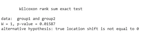
Example: The Mann-Whitney U Test compares two independent groups to determine if they come from the same distribution. We are comparing group1 and group2 to see if there is a significant difference in their distributions.
R
group1 <- c(23, 21, 18, 25, 30)
group2 <- c(35, 37, 29, 40, 42)
result <- wilcox.test(group1, group2)
print(result)
Output:
 Output
A p-value of 0.016 indicates a significant difference between group1 and group2.
3. Wilcoxon Signed-Rank Test
Wilcoxon Signed-Rank test compares the differences between two related samples or repeated measurements on a single sample, typically when the data are ordinal or continuous but not normally distributed.
Syntax:
wilcox.test()
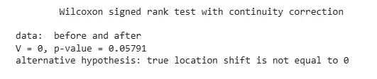
Example: The Wilcoxon Signed-Rank Test compares two related samples or matched pairs. Here, we compare before and after treatment values to see if there is a significant difference.
R
before <- c(12, 10, 15, 14, 18)
after <- c(15, 13, 16, 19, 20)
result <- wilcox.test(before, after, paired = TRUE)
print(result)
Output:
 Output
A p-value of 0.05791 suggests that the difference between the before and after values is not statistically significant at the 0.05 level.
4. Kruskal-Wallis H Test
The Kruskal-Wallis test is an extension of the Mann-Whitney U test for more than two groups. It is used to determine if there are statistically significant differences between two or more independent groups.
Syntax:
kruskal.test()
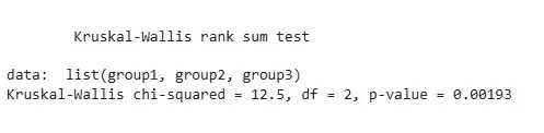
Example: The Kruskal-Wallis Test is used to compare three or more independent groups. In this case, we compare group1, group2, and group3 to see if there are any significant differences.
R
group1 <- c(4, 5, 6, 7, 8)
group2 <- c(9, 10, 11, 12, 13)
group3 <- c(14, 15, 16, 17, 18)
result <- kruskal.test(list(group1, group2, group3))
print(result)
Output:
 Output
A p-value of 0.105 suggests no significant difference between the groups.
5. Friedman Test
The Friedman test is used to detect differences in treatments across multiple test attempts. It is an extension of the Wilcoxon Signed-Rank test for more than two groups, applied to repeated measures or matched data.
Syntax:
friedman.test()
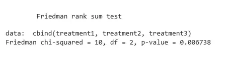
Example: The Friedman Test is used to compare repeated measures across three or more conditions or time points for the same subjects. We compare treatment1, treatment2, and treatment3 here.
R
treatment1 <- c(15, 16, 14, 13, 12)
treatment2 <- c(20, 19, 21, 18, 16)
treatment3 <- c(17, 18, 19, 16, 15)
result <- friedman.test(cbind(treatment1, treatment2, treatment3))
print(result)
Output:
 Output
A p-value of 0.3006 suggests no significant difference between the treatments.
6. Chi-Square Test for Independence
Chi-Square test is used to examine the relationship between two categorical variables. It tests whether the distribution of sample categorical data matches an expected distribution.
Syntax:
chisq.test()
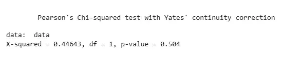
Example: The Chi-Square Test is used to examine the association between categorical variables. We test if there is independence between two variables represented by a contingency table.
R
data <- matrix(c(10, 20, 30, 40), nrow = 2)
result <- chisq.test(data)
print(result)
Output:
 Output
A p-value of 0.4795 suggests no significant association between the categorical variables.
7. Spearman’s Rank Correlation
Spearman’s Rank Correlation test is used to assess the strength and direction of the association between two variables that are ordinal or continuous but not normally distributed.
Syntax:
cor.test()
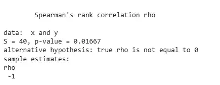
Example: Spearman's Rank Correlation assesses the strength and direction of association between two ranked variables. Here, we assess the correlation between x and y.
R
x <- c(1, 2, 3, 4, 5)
y <- c(5, 4, 3, 2, 1)
result <- cor.test(x, y, method = "spearman")
print(result)
Output:
 Output
A p-value of 0.016 indicates a perfect negative correlation between x and y.
8. Kolmogorov-Smirnov Test
The Kolmogorov-Smirnov test is used to compare the distributions of two samples. It can also be used to compare a sample against a known distribution.
Syntax:
ks.test()
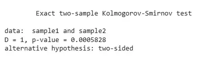
Example: The Kolmogorov-Smirnov test compares the distributions of two samples to see if they come from the same distribution. We are testing if sample1 and sample2 differ significantly in their distributions.
R
sample1 <- c(12, 15, 14, 10, 19, 18, 21)
sample2 <- c(23, 24, 25, 26, 22, 27, 28)
result <- ks.test(sample1, sample2)
print(result)
Output:
 Output
A p-value of 0.0625 suggests no significant difference between sample1 and sample2.