Big O notation is a powerful tool used in computer science to describe the time complexity or space complexity of algorithms. Big-O is a way to express the upper bound of an algorithm’s time or space complexity.
- Describes the asymptotic behavior (order of growth of time or space in terms of input size) of a function, not its exact value.
- Can be used to compare the efficiency of different algorithms or data structures.
- It provides an upper limit on the time taken by an algorithm in terms of the size of the input. We mainly consider the worst case scenario of the algorithm to find its time complexity in terms of Big O
- It’s denoted as O(f(n)), where f(n) is a function that represents the number of operations (steps) that an algorithm performs to solve a problem of size n.

Big O Definition
Given two functions f(n) and g(n), we say that f(n) is O(g(n)) if there exist constants c > 0 and n0 >= 0 such that f(n) <= c*g(n) for all n >= n0.
In simpler terms, f(n) is O(g(n)) if f(n) grows no faster than c*g(n) for all n >= n0 where c and n0 are constants.

Importance of Big O Notation
Big O notation is a mathematical notation used to find an upper bound on time taken by an algorithm or data structure. It provides a way to compare the performance of different algorithms and data structures, and to predict how they will behave as the input size increases.
Big O notation is important for several reasons:
- Big O Notation is important because it helps analyze the efficiency of algorithms.
- It provides a way to describe how the runtime or space requirements of an algorithm grow as the input size increases.
- Allows programmers to compare different algorithms and choose the most efficient one for a specific problem.
- Helps in understanding the scalability of algorithms and predicting how they will perform as the input size grows.
- Enables developers to optimize code and improve overall performance.
A Quick Way to find Big O of an Expression
- Ignore the lower order terms and consider only highest order term.
- Ignore the constant associated with the highest order term.
Example 1: f(n) = 3n2 + 2n + 1000Logn + 5000
After ignoring lower order terms, we get the highest order term as 3n2
After ignoring the constant 3, we get n2
Therefore the Big O value of this expression is O(n2)
Example 2 : f(n) = 3n3 + 2n2 + 5n + 1
Dominant Term: 3n3
Order of Growth: Cubic (n3)
Big O Notation: O(n3)
Properties of Big O Notation
Below are some important Properties of Big O Notation:
1. Reflexivity
For any function f(n), f(n) = O(f(n)).
Example:
f(n) = n2, then f(n) = O(n2).
2. Transitivity
If f(n) = O(g(n)) and g(n) = O(h(n)), then f(n) = O(h(n)).
Example:
If f(n) = n^2, g(n) = n^3, and h(n) = n^4, then f(n) = O(g(n)) and g(n) = O(h(n)).
Therefore, by transitivity, f(n) = O(h(n)).
3. Constant Factor
For any constant c > 0 and functions f(n) and g(n), if f(n) = O(g(n)), then cf(n) = O(g(n)).
Example:
f(n) = n, g(n) = n2. Then f(n) = O(g(n)). Therefore, 2f(n) = O(g(n)).
4. Sum Rule
If f(n) = O(g(n)) and h(n) = O(k(n)), then f(n) + h(n) = O(max( g(n), k(n) ) When combining complexities, only the largest term dominates.
Example:
f(n) = n2, h(n) = n3. Then , f(n) + h(n) = O(max(n2 + n3) = O ( n3)
5. Product Rule
If f(n) = O(g(n)) and h(n) = O(k(n)), then f(n) * h(n) = O(g(n) * k(n)).
Example:
f(n) = n, g(n) = n2, h(n) = n3, k(n) = n4. Then f(n) = O(g(n)) and h(n) = O(k(n)). Therefore, f(n) * h(n) = O(g(n) * k(n)) = O(n6).
6. Composition Rule
If f(n) = O(g(n)), then f(h(n)) = O(g(h(n))).
Example:
If f(n) = n^2, g(n) = n^3 and h(n) = log n, then by composition rule f(h(n))=O(g(h(n))). Therefore, (log n)^2=O((log n)^3).
Common Big-O Notations
Big-O notation is a way to measure the time and space complexity of an algorithm. It describes the upper bound of the complexity in the worst-case scenario. Let’s look into the different types of time complexities:
1. Linear Time Complexity: Big O(n) Complexity
Linear time complexity means that the running time of an algorithm grows linearly with the size of the input.
For example, consider an algorithm that traverses through an array to find a specific element:
Code Snippet
bool findElement(int arr[], int n, int key)
{
    for (int i = 0; i < n; i++) {
        if (arr[i] == key) {
            return true;
        }
    }
    return false;
}
2. Logarithmic Time Complexity: Big O(log n) Complexity
Logarithmic time complexity means that the running time of an algorithm is proportional to the logarithm of the input size.
For example, a binary search algorithm has a logarithmic time complexity:
Code Snippet
int binarySearch(int arr[], int l, int r, int x)
{
    if (r >= l) {
        int mid = l + (r - l) / 2;
        if (arr[mid] == x)
            return mid;
        if (arr[mid] > x)
            return binarySearch(arr, l, mid - 1, x);
        return binarySearch(arr, mid + 1, r, x);
    }
    return -1;
}
3. Quadratic Time Complexity: Big O(n2) Complexity
Quadratic time complexity means that the running time of an algorithm is proportional to the square of the input size.
For example, a simple bubble sort algorithm has a quadratic time complexity:
Code Snippet
void bubbleSort(int arr[], int n)
{
    for (int i = 0; i < n - 1; i++) {
        for (int j = 0; j < n - i - 1; j++) {
            if (arr[j] > arr[j + 1]) {
                swap(&arr[j], &arr[j + 1]);
            }
        }
    }
}
4. Cubic Time Complexity: Big O(n3) Complexity
Cubic time complexity means that the running time of an algorithm is proportional to the cube of the input size.
For example, a naive matrix multiplication algorithm has a cubic time complexity:
Code Snippet
void multiply(int mat1[][N], int mat2[][N], int res[][N])
{
    for (int i = 0; i < N; i++) {
        for (int j = 0; j < N; j++) {
            res[i][j] = 0;
            for (int k = 0; k < N; k++)
                res[i][j] += mat1[i][k] * mat2[k][j];
        }
    }
}
5. Polynomial Time Complexity: Big O(nk) Complexity
Polynomial time complexity refers to the time complexity of an algorithm that can be expressed as a polynomial function of the input size n. In Big O notation, an algorithm is said to have polynomial time complexity if its time complexity is O(nk), where k is a constant and represents the degree of the polynomial.
Algorithms with polynomial time complexity are generally considered efficient, as the running time grows at a reasonable rate as the input size increases. Common examples of algorithms with polynomial time complexity include linear time complexity O(n), quadratic time complexity O(n2), and cubic time complexity O(n3).
6. Exponential Time Complexity: Big O(2n) Complexity
Exponential time complexity means that the running time of an algorithm doubles with each addition to the input data set.
For example, the problem of generating all subsets of a set is of exponential time complexity:
Code Snippet
void generateSubsets(int arr[], int n)
{
    for (int i = 0; i < (1 << n); i++) {
        for (int j = 0; j < n; j++) {
            if (i & (1 << j)) {
                cout << arr[j] << " ";
            }
        }
        cout << endl;
    }
}
7. Factorial Time Complexity: Big O(n!) Complexity
Factorial time complexity means that the running time of an algorithm grows factorially with the size of the input. This is often seen in algorithms that generate all permutations of a set of data.
Here’s an example of a factorial time complexity algorithm, which generates all permutations of an array:
Code Snippet
void permute(int* a, int l, int r)
{
    if (l == r) {
        for (int i = 0; i <= r; i++) {
            cout << a[i] << " ";
        }
        cout << endl;
    }
    else {
        for (int i = l; i <= r; i++) {
            swap(a[l], a[i]);
            permute(a, l + 1, r);
            swap(a[l], a[i]); // backtrack
        }
    }
}
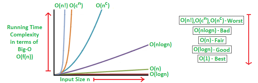
If we plot the most common Big O notation examples, we would have graph like this:
Mathematical Examples of Runtime Analysis
Below table illustrates the runtime analysis of different orders of algorithms as the input size (n) increases.
| n | log(n) | n | n * log(n) | n^2 | 2^n | n! |
|---|
| 10 | 1 | 10 | 10 | 100 | 1024 | 3628800 |
| 20 | 2.996 | 20 | 59.9 | 400 | 1048576 | 2.432902e+1818 |
Algorithmic Examples of Runtime Analysis
Below table categorizes algorithms based on their runtime complexity and provides examples for each type.
| Type | Notation | Example Algorithms |
|---|
| Logarithmic | O(log n) | Binary Search |
| Linear | O(n) | Linear Search |
| Superlinear | O(n log n) | Heap Sort, Merge Sort |
| Polynomial | O(n^c) | Strassen’s Matrix Multiplication, Bubble Sort, Selection Sort, Insertion Sort, Bucket Sort |
| Exponential | O(c^n) | Tower of Hanoi |
| Factorial | O(n!) | Determinant Expansion by Minors, Brute force Search algorithm for Traveling Salesman Problem |
Algorithm Classes with Number of Operations
Below are the classes of algorithms and their number of operations assuming that there are no constants.
Big O Notation Classes | f(n) | Big O Analysis (number of operations) for n = 10 |
|---|
constant | O(1) | 1 |
|---|
logarithmic | O(logn) | 3.32 |
|---|
linear | O(n) | 10 |
|---|
O(nlogn) | O(nlogn) | 33.2 |
|---|
quadratic | O(n2) | 102 |
|---|
cubic | O(n3) | 103 |
|---|
exponential | O(2n) | 1024 |
|---|
factorial | O(n!) | 10! |
|---|
Comparison of Big O Notation, Big Ω (Omega) Notation, and Big θ (Theta) Notation
Below is a table comparing Big O notation, Ω (Omega) notation, and θ (Theta) notation:
| Notation | Definition | Explanation |
|---|
| Big O (O) | f(n) ≤ C * g(n) for all n ≥ n0 | Describes the upper bound of the algorithm's running time. Used most of the time. |
| Ω (Omega) | f(n) ≥ C * g(n) for all n ≥ n0 | Describes the lower bound of the algorithm's running time . Used less |
| θ (Theta) | C1 * g(n) ≤ f(n) ≤ C2 * g(n) for n ≥ n0 | Describes both the upper and lower bounds of the algorithm's running time. Also used a lot more and preferred over Big O if we can find an exact bound. |
In each notation:
- f(n) represents the function being analyzed, typically the algorithm's time complexity.
- g(n) represents a specific function that bounds f(n).
- C, C1, and C2 are constants.
- n0 is the minimum input size beyond which the inequality holds.
These notations are used to analyze algorithms based on their worst-case (Big O), best-case (Ω) and average-case (θ) scenarios.
Related Article: