|
|
|
| CARVIEW |


Open Cryptochat - A Tutorial

Cryptography is important. Without encryption, the internet as we know it would not be possible - data sent online would be as vulnerable to interception as a message shouted across a crowded room. Cryptography is also a major topic in current events, increasingly playing a central role in law enforcement investigations and government legislation.
Encryption is an invaluable tool for journalists, activists, nation-states, businesses, and everyday people who need to protect their data from the ever-present threat of hackers, spies, and advertising agencies.
An understanding of how to utilize strong encryption is essential for modern software development. We will not be delving much into the underlying math and theory of cryptography for this tutorial; instead, the focus will be on how to harness these techniques for your own applications.
In this tutorial, we will walk through the basic concepts and implementation of an end-to-end 2048-bit RSA encrypted messenger. We'll be utilizing Vue.js for coordinating the frontend functionality along with a Node.js backend using Socket.io for sending messages between users.
- Live Preview - https://chat.patricktriest.com
- Github Repository - https://github.com/triestpa/Open-Cryptochat
The concepts that we are covering in this tutorial are implemented in Javascript and are mostly intended to be platform-agnostic. We will be building a traditional browser-based web app, but you can adapt this code to work within a pre-built desktop (using Electron) or mobile ( React Native, Ionic, Cordova) application binary if you are concerned about browser-based application security.[1] Likewise, implementing similar functionality in another programming language should be relatively straightforward since most languages have reputable open-source encryption libraries available; the base syntax will change but the core concepts remain universal.
Disclaimer - This is meant to be a primer in end-to-end encryption implementation, not a definitive guide to building the Fort Knox of browser chat applications. I've worked to provide useful information on adding cryptography to your Javascript applications, but I cannot 100% guarantee the security of the resulting app. There's a lot that can go wrong at all stages of the process, especially at the stages not covered by this tutorial such as setting up web hosting and securing the server(s). If you are a security expert, and you find vulnerabilities in the tutorial code, please feel free to reach out to me by email (patrick.triest@gmail.com) or in the comments section below.
1 - Project Setup
1.0 - Install Dependencies
You'll need to have Node.js (version 6 or higher) installed in order to run the backend for this app.
Create an empty directory for the project and add a package.json file with the following contents.
{
  "name": "open-cryptochat",
  "version": "1.0.0",
  "node":"8.1.4",
  "license": "MIT",
  "author": "patrick.triest@gmail.com",
  "description": "End-to-end RSA-2048 encrypted chat application.",
  "main": "app.js",
  "engines": {
    "node": ">=7.6"
  },
  "scripts": {
    "start": "node app.js"
  },
  "dependencies": {
    "express": "4.15.3",
    "socket.io": "2.0.3"
  }
}
Run npm install on the command line to install the two Node.js dependencies.
1.1 - Create Node.js App
Create a file called app.js, and add the following contents.
const express = require('express')
// Setup Express server
const app = express()
const http = require('http').Server(app)
// Attach Socket.io to server
const io = require('socket.io')(http)
// Serve web app directory
app.use(express.static('public'))
// INSERT SOCKET.IO CODE HERE
// Start server
const port = process.env.PORT || 3000
http.listen(port, () => {
  console.log(`Chat server listening on port ${port}.`)
})
This is the core server logic. Right now, all it will do is start a server and make all of the files in the local /public directory accessible to web clients.
In production, I would strongly recommend serving your frontend code separately from the Node.js app, using battle-hardened server software such Apache and Nginx, or hosting the website on file storage service such as AWS S3. For this tutorial, however, using the Express static file server is the simplest way to get the app running.
1.2 - Add Frontend
Create a new directory called public. This is where we'll put all of the frontend web app code.
1.2.0 - Add HTML Template
Create a new file, /public/index.html, and add these contents.
<!DOCTYPE html>
<html lang="en">
  <head>
    <meta charset="utf-8">
    <title>Open Cryptochat</title>
    <meta name="description" content="A minimalist, open-source, end-to-end RSA-2048 encrypted chat application.">
    <meta name="viewport" content="width=device-width, initial-scale=1, maximum-scale=1, user-scalable=no">
    <link href="https://fonts.googleapis.com/css?family=Montserrat:300,400" rel="stylesheet">
    <link href="https://fonts.googleapis.com/css?family=Roboto+Mono" rel="stylesheet">
    <link href="/styles.css" rel="stylesheet">
  </head>
  <body>
    <div id="vue-instance">
      <!-- Add Chat Container Here -->
      <div class="info-container full-width">
        <!-- Add Room UI Here -->
        <div class="notification-list" ref="notificationContainer">
          <h1>NOTIFICATION LOG</h1>
          <div class="notification full-width" v-for="notification in notifications">
            <div class="notification-timestamp">{{ notification.timestamp }}</div>
            <div class="notification-message">{{ notification.message }}</div>
          </div>
        </div>
        <div class="flex-fill"></div>
        <!-- Add Encryption Key UI Here -->
      </div>
      <!-- Add Bottom Bar Here -->
    </div>
    <script src="https://cdnjs.cloudflare.com/ajax/libs/vue/2.4.1/vue.min.js"></script>
    <script src="https://cdnjs.cloudflare.com/ajax/libs/socket.io/2.0.3/socket.io.slim.js"></script>
    <script src="https://cdnjs.cloudflare.com/ajax/libs/immutable/3.8.1/immutable.min.js"></script>
    <script src="/page.js"></script>
  </body>
</html>
This template sets up the baseline HTML structure and downloads the client-side JS dependencies. It will also display a simple list of notifications once we add the client-side JS code.
1.2.1 - Create Vue.js App
Add the following contents to a new file, /public/page.js.
/** The core Vue instance controlling the UI */
const vm = new Vue ({
  el: '#vue-instance',
  data () {
    return {
      cryptWorker: null,
      socket: null,
      originPublicKey: null,
      destinationPublicKey: null,
      messages: [],
      notifications: [],
      currentRoom: null,
      pendingRoom: Math.floor(Math.random() * 1000),
      draft: ''
    }
  },
  created () {
    this.addNotification('Hello World')
  },
  methods: {
    /** Append a notification message in the UI */
    addNotification (message) {
      const timestamp = new Date().toLocaleTimeString()
      this.notifications.push({ message, timestamp })
    },
  }
})
This script will initialize the Vue.js application and will add a "Hello World" notification to the UI.
1.2.2 - Add Styling
Create a new file, /public/styles.css and paste in the following stylesheet.
/* Global */
:root {
  --black: #111111;
  --light-grey: #d6d6d6;
  --highlight: yellow;
}
body {
  background: var(--black);
  color: var(--light-grey);
  font-family: 'Roboto Mono', monospace;
  height: 100vh;
  display: flex;
  padding: 0;
  margin: 0;
}
div { box-sizing: border-box; }
input, textarea, select { font-family: inherit; font-size: small; }
textarea:focus, input:focus { outline: none; }
.full-width { width: 100%; }
.green { color: green; }
.red { color: red; }
.yellow { color: yellow; }
.center-x { margin: 0 auto; }
.center-text { width: 100%; text-align: center; }
h1, h2, h3 { font-family: 'Montserrat', sans-serif; }
h1 { font-size: medium; }
h2 { font-size: small; font-weight: 300; }
h3 { font-size: x-small; font-weight: 300; }
p { font-size: x-small; }
.clearfix:after {
   visibility: hidden;
   display: block;
   height: 0;
   clear: both;
}
#vue-instance {
  display: flex;
  flex-direction: row;
  flex: 1 0 100%;
  overflow-x: hidden;
}
/** Chat Window **/
.chat-container {
  flex: 0 0 60%;
  word-wrap: break-word;
  overflow-x: hidden;
  overflow-y: scroll;
  padding: 6px;
  margin-bottom: 50px;
}
.message > p { font-size: small; }
.title-header > p {
  font-family: 'Montserrat', sans-serif;
  font-weight: 300;
}
/* Info Panel */
.info-container {
  flex: 0 0 40%;
  border-left: solid 1px var(--light-grey);
  padding: 12px;
  overflow-x: hidden;
  overflow-y: scroll;
  margin-bottom: 50px;
  position: relative;
  justify-content: space-around;
  display: flex;
  flex-direction: column;
}
.divider {
  padding-top: 1px;
  max-height: 0px;
  min-width: 200%;
  background: var(--light-grey);
  margin: 12px -12px;
  flex: 1 0;
}
.notification-list {
  display: flex;
  flex-direction: column;
  overflow: scroll;
  padding-bottom: 24px;
  flex: 1 0 40%;
}
.notification {
  font-family: 'Montserrat', sans-serif;
  font-weight: 300;
  font-size: small;
  padding: 4px 0;
  display: inline-flex;
}
.notification-timestamp {
  flex: 0 0 20%;
  padding-right: 12px;
}
.notification-message { flex: 0 0 80%; }
.notification:last-child {
  margin-bottom: 24px;
}
.keys {
  display: block;
  font-size: xx-small;
  overflow-x: hidden;
  overflow-y: scroll;
}
.keys > .divider {
  width: 75%;
  min-width: 0;
  margin: 16px auto;
}
.key { overflow: scroll; }
.room-select {
  display: flex;
  min-height: 24px;
  font-family: 'Montserrat', sans-serif;
  font-weight: 300;
}
#room-input {
    flex: 0 0 60%;
    background: none;
    border: none;
    border-bottom: 1px solid var(--light-grey);
    border-top: 1px solid var(--light-grey);
    border-left: 1px solid var(--light-grey);
    color: var(--light-grey);
    padding: 4px;
}
.yellow-button {
  flex: 0 0 30%;
  background: none;
  border: 1px solid var(--highlight);
  color: var(--highlight);
  cursor: pointer;
}
.yellow-button:hover {
  background: var(--highlight);
  color: var(--black);
}
.yellow > a { color: var(--highlight); }
.loader {
    border: 4px solid black;
    border-top: 4px solid var(--highlight);
    border-radius: 50%;
    width: 48px;
    height: 48px;
    animation: spin 2s linear infinite;
}
@keyframes spin {
    0% { transform: rotate(0deg); }
    100% { transform: rotate(360deg); }
}
/* Message Input Bar */
.message-input {
  background: none;
  border: none;
  color: var(--light-grey);
  width: 90%;
}
.bottom-bar {
  border-top: solid 1px var(--light-grey);
  background: var(--black);
  position: fixed;
  bottom: 0;
  left: 0;
  padding: 12px;
  height: 48px;
}
.message-list {
  margin-bottom: 40px;
}
We won't really be going into the CSS, but I can assure you that it's all fairly straight-forward.
For the sake of simplicity, we won't bother to add a build system to our frontend. A build system, in my opinion, is just not really necessary for an app this simple (the total gzipped payload of the completed app is under 100kb). You are very welcome (and encouraged, since it will allow the app to be backwards compatible with outdated browsers) to add a build system such as Webpack, Gulp, or Rollup to the application if you decide to fork this code into your own project.
1.3 - Try it out
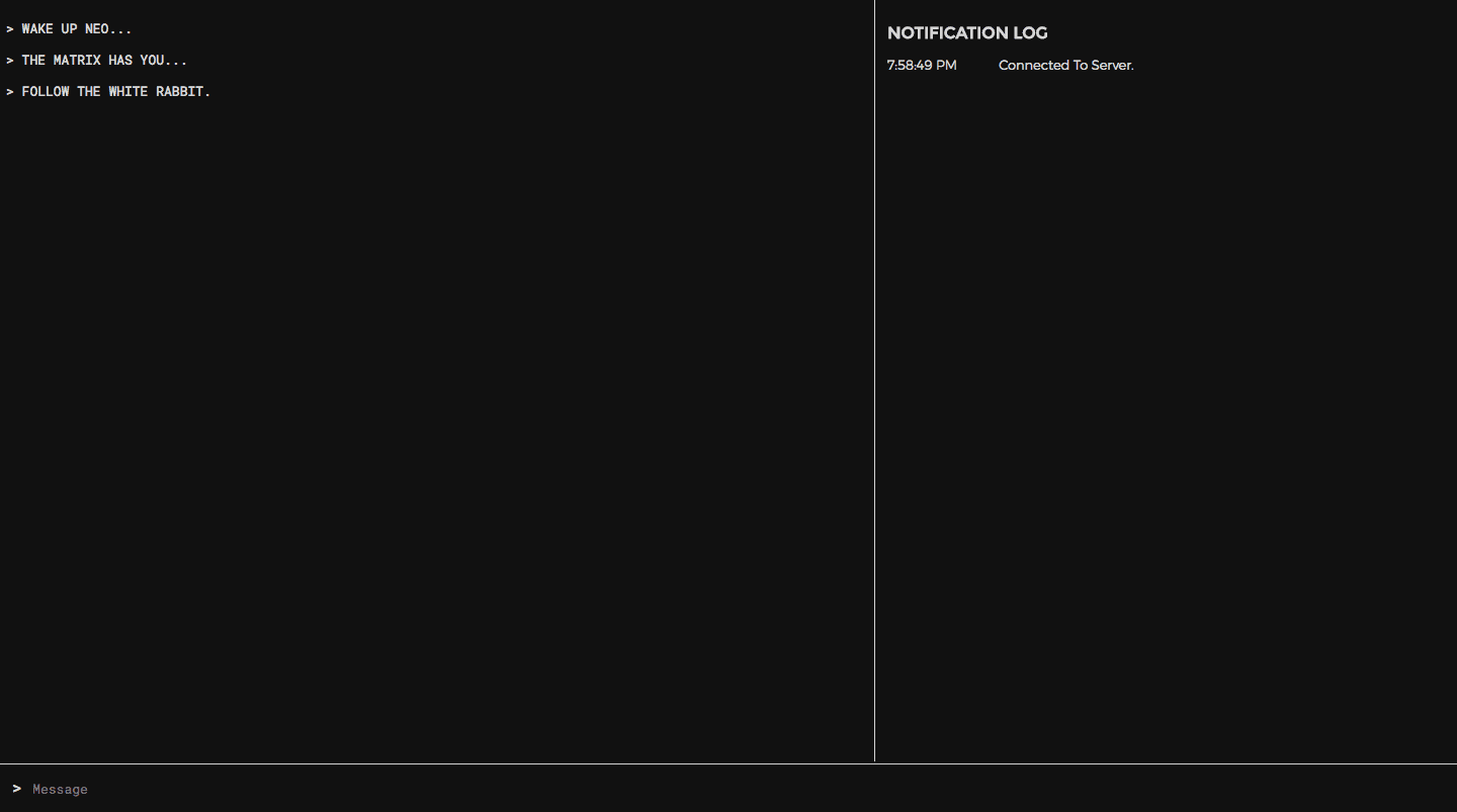
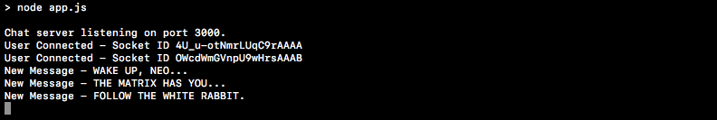
Try running npm start on the command-line. You should see the command-line output Chat server listening on port 3000.. Open https://localhost:3000 in your browser, and you should see a very dark, empty web app displaying "Hello World" on the right side of the page.

2 - Basic Messaging
Now that the baseline project scaffolding is in place, we'll start by adding basic (unencrypted) real-time messaging.
2.0 - Setup Server-Side Socket Listeners
In /app.js, add the follow code directly below the // INSERT SOCKET.IO CODE HERE marker.
/** Manage behavior of each client socket connection */
io.on('connection', (socket) => {
  console.log(`User Connected - Socket ID ${socket.id}`)
  // Store the room that the socket is connected to
  let currentRoom = 'DEFAULT'
  /** Process a room join request. */
  socket.on('JOIN', (roomName) => {
    socket.join(currentRoom)
    // Notify user of room join success
    io.to(socket.id).emit('ROOM_JOINED', currentRoom)
    // Notify room that user has joined
    socket.broadcast.to(currentRoom).emit('NEW_CONNECTION', null)
  })
  /** Broadcast a received message to the room */
  socket.on('MESSAGE', (msg) => {
    console.log(`New Message - ${msg.text}`)
    socket.broadcast.to(currentRoom).emit('MESSAGE', msg)
  })
})
This code-block will create a connection listener that will manage any clients who connect to the server from the front-end application. Currently, it just adds them to a DEFAULT chat room, and retransmits any message that it receives to the rest of the users in the room.
2.1 - Setup Client-Side Socket Listeners
Within the frontend, we'll add some code to connect to the server. Replace the created function in /public/page.js with the following.
created () {
  // Initialize socket.io
  this.socket = io()
  this.setupSocketListeners()
},
Next, we'll need to add a few custom functions to manage the client-side socket connection and to send/receive messages. Add the following to /public/page.js inside the methods block of the Vue app object.
/** Setup Socket.io event listeners */
setupSocketListeners () {
  // Automatically join default room on connect
  this.socket.on('connect', () => {
    this.addNotification('Connected To Server.')
    this.joinRoom()
  })
  // Notify user that they have lost the socket connection
  this.socket.on('disconnect', () => this.addNotification('Lost Connection'))
  // Display message when recieved
  this.socket.on('MESSAGE', (message) => {
    this.addMessage(message)
  })
},
/** Send the current draft message */
sendMessage () {
  // Don't send message if there is nothing to send
  if (!this.draft || this.draft === '') { return }
  const message = this.draft
  // Reset the UI input draft text
  this.draft = ''
  // Instantly add message to local UI
  this.addMessage(message)
  // Emit the message
  this.socket.emit('MESSAGE', message)
},
/** Join the chatroom */
joinRoom () {
  this.socket.emit('JOIN')
},
/** Add message to UI */
addMessage (message) {
  this.messages.push(message)
},
2.2 - Display Messages in UI
Finally, we'll need to provide a UI to send and display messages.
In order to display all messages in the current chat, add the following to /public/index.html after the <!-- Add Chat Container Here --> comment.
<div class="chat-container full-width" ref="chatContainer">
  <div class="message-list">
    <div class="message full-width" v-for="message in messages">
      <p>
      > {{ message }}
      </p>
    </div>
  </div>
</div>
To add a text input bar for the user to write messages in, add the following to /public/index.html, after the <!-- Add Bottom Bar Here --> comment.
<div class="bottom-bar full-width">
  > <input class="message-input" type="text" placeholder="Message" v-model="draft" @keyup.enter="sendMessage()">
</div>
Now, restart the server and open https://localhost:3000 in two separate tabs/windows. Try sending messages back and forth between the tabs. In the command-line, you should be able to see a server log of messages being sent.
Encryption 101
Cool, now we have a real-time messaging application. Before adding end-to-end encryption, it's important to have a basic understanding of how asymmetric encryption works.
Symetric Encryption & One Way Functions
Let's say we're trading secret numbers. We're sending the numbers through a third party, but we don't want the third party to know which number we are exchanging.
In order to accomplish this, we'll exchange a shared secret first - let's use 7.
To encrypt the message, we'll first multiply our shared secret (7) by a random number n, and add a value x to the result. In this equation, x represents the number that we want to send and y represents the encrypted result.
(7 * n) + x = y
We can then use modular arithmetic in order to transform an encrypted input into the decrypted output.
y mod 7 = x
Here, y as the exposed (encrypted) message and x is the original unencrypted message.
If one of us wants to exchange the number 2, we could compute (7*4) + 2 and send 30 as a message. We both know the secret key (7), so we'll both be able to calculate 30 mod 7 and determine that 2 was the original number.
The original number (2), is effectively hidden from anyone listening in the middle since the only message passed between us was 30. If a third party is able to retrieve both the unencrypted result (30) and the encrypted value (2), they would still not know the value of the secret key. In this example, 30 mod 14 and 30 mod 28 are also equal to 2, so an interceptor could not know for certain whether the secret key is 7, 14, or 28, and therefore could not dependably decipher the next message.
Modulo is thus considered a "one-way" function since it cannot be trivially reversed.
Modern encryption algorithms are, to vastly simplify and generalize, very complex applications of this general principle. Through the use of large prime numbers, modular exponentiation, long private keys, and multiple rounds of cipher transformations, these algorithms generally take a very inconvenient amount a time (1+ million years) to crack.
Quantum computers could, theoretically, crack these ciphers more quickly. You can read more about this here. This technology is still in its infancy, so we probably don't need to worry about encrypted data being compromised in this manner just yet.
The above example assumes that both parties were able to exchange a secret (in this case 7) ahead of time. This is called symmetric encryption since the same secret key is used for both encrypting and decrypting the message. On the internet, however, this is often not a viable option - we need a way to send encrypted messages without requiring offline coordination to decide on a shared secret. This is where asymmetric encryption comes into play.
Public Key Cryptography
In contrast to symmetric encryption, public key cryptography (asymmetric encryption) uses pairs of keys (one public, one private) instead of a single shared secret - public keys are for encrypting data, and private keys are for decrypting data.
A public key is like an open box with an unbreakable lock. If someone wants to send you a message, they can place that message in your public box, and close the lid to lock it. The message can now be sent, to be delivered by an untrusted party without needing to worry about the contents being exposed. Once I receive the box, I'll unlock it with my private key - the only existing key which can open that box.
Exchanging public keys is like exchanging those boxes - each private key is kept safe with the original owner, so the contents of the box are safe in transit.
This is, of course, a bare-bones simplification of how public key cryptography works. If you're curious to learn more (especially regarding the history and mathematical basis for these techniques) I would strongly recommend starting with these two videos.
3 - Crypto Web Worker
Cryptographic operations tend to be computationally intensive. Since Javascript is single-threaded, doing these operations on the main UI thread will cause the browser to freeze for a few seconds.
Wrapping the operations in a promise will not help, since promises are for managing asynchronous operations on a single-thread, and do not provide any performance benefit for computationally intensive tasks.
In order to keep the application performant, we will use a Web Worker to perform cryptographic computations on a separate browser thread. We'll be using JSEncrypt, a reputable Javascript RSA implementation originating from Stanford. Using JSEncrypt, we'll create a few helper functions for encryption, decryption, and key pair generation.
3.0 - Create Web Worker To Wrap the JSencrypt Methods
Add a new file called crypto-worker.js in the public directory. This file will store our web worker code in order to perform encryption operations on a separate browser thread.
self.window = self // This is required for the jsencrypt library to work within the web worker
// Import the jsencrypt library
self.importScripts('https://cdnjs.cloudflare.com/ajax/libs/jsencrypt/2.3.1/jsencrypt.min.js');
let crypt = null
let privateKey = null
/** Webworker onmessage listener */
onmessage = function(e) {
  const [ messageType, messageId, text, key ] = e.data
  let result
  switch (messageType) {
    case 'generate-keys':
      result = generateKeypair()
      break
    case 'encrypt':
      result = encrypt(text, key)
      break
    case 'decrypt':
      result = decrypt(text)
      break
  }
  // Return result to the UI thread
  postMessage([ messageId, result ])
}
/** Generate and store keypair */
function generateKeypair () {
  crypt = new JSEncrypt({default_key_size: 2056})
  privateKey = crypt.getPrivateKey()
  // Only return the public key, keep the private key hidden
  return crypt.getPublicKey()
}
/** Encrypt the provided string with the destination public key */
function encrypt (content, publicKey) {
  crypt.setKey(publicKey)
  return crypt.encrypt(content)
}
/** Decrypt the provided string with the local private key */
function decrypt (content) {
  crypt.setKey(privateKey)
  return crypt.decrypt(content)
}
This web worker will receive messages from the UI thread in the onmessage listener, perform the requested operation, and post the result back to the UI thread. The private encryption key is never directly exposed to the UI thread, which helps to mitigate the potential for key theft from a cross-site scripting (XSS) attack.
3.1 - Configure Vue App To Communicate with Web Worker
Next, we'll configure the UI controller to communicate with the web worker. Sequential call/response communications using event listeners can be painful to synchronize. To simplify this, we'll create a utility function that wraps the entire communication lifecycle in a promise. Add the following code to the methods block in /public/page.js.
/** Post a message to the web worker and return a promise that will resolve with the response.  */
getWebWorkerResponse (messageType, messagePayload) {
  return new Promise((resolve, reject) => {
    // Generate a random message id to identify the corresponding event callback
    const messageId = Math.floor(Math.random() * 100000)
    // Post the message to the webworker
    this.cryptWorker.postMessage([messageType, messageId].concat(messagePayload))
    // Create a handler for the webworker message event
    const handler = function (e) {
      // Only handle messages with the matching message id
      if (e.data[0] === messageId) {
        // Remove the event listener once the listener has been called.
        e.currentTarget.removeEventListener(e.type, handler)
        // Resolve the promise with the message payload.
        resolve(e.data[1])
      }
    }
    // Assign the handler to the webworker 'message' event.
    this.cryptWorker.addEventListener('message', handler)
  })
}
This code will allow us to trigger an operation on the web worker thread and receive the result in a promise. This can be a very useful helper function in any project that outsources call/response processing to web workers.
4 - Key Exchange
In our app, the first step will be generating a public-private key pair for each user. Then, once the users are in the same chat, we will exchange public keys so that each user can encrypt messages which only the other user can decrypt. Hence, we will always encrypt messages using the recipient's public key, and we will always decrypt messages using the recipient's private key.
4.0 - Add Server-Side Socket Listener To Transmit Public Keys
On the server-side, we'll need a new socket listener that will receive a public-key from a client and re-broadcast this key to the rest of the room. We'll also add a listener to let clients know when someone has disconnected from the current room.
Add the following listeners to /app.js within the io.on('connection', (socket) => { ... } callback.
/** Broadcast a new publickey to the room */
socket.on('PUBLIC_KEY', (key) => {
  socket.broadcast.to(currentRoom).emit('PUBLIC_KEY', key)
})
/** Broadcast a disconnection notification to the room */
socket.on('disconnect', () => {
  socket.broadcast.to(currentRoom).emit('USER_DISCONNECTED', null)
})
4.1 - Generate Key Pair
Next, we'll replace the created function in /public/page.js to initialize the web worker and generate a new key pair.
async created () {
  this.addNotification('Welcome! Generating a new keypair now.')
  // Initialize crypto webworker thread
  this.cryptWorker = new Worker('crypto-worker.js')
  // Generate keypair and join default room
  this.originPublicKey = await this.getWebWorkerResponse('generate-keys')
  this.addNotification('Keypair Generated')
  // Initialize socketio
  this.socket = io()
  this.setupSocketListeners()
},
We are using the async/await syntax to receive the web worker promise result with a single line of code.
4.2 - Add Public Key Helper Functions
We'll also add a few new functions to /public/page.js for sending the public key, and to trim down the key to a human-readable identifier.
/** Emit the public key to all users in the chatroom */
sendPublicKey () {
  if (this.originPublicKey) {
    this.socket.emit('PUBLIC_KEY', this.originPublicKey)
  }
},
/** Get key snippet for display purposes */
getKeySnippet (key) {
  return key.slice(400, 416)
},
4.3 - Send and Receive Public Key
Next, we'll add some listeners to the client-side socket code, in order to send the local public key whenever a new user joins the room, and to save the public key sent by the other user.
Add the following to /public/page.js within the setupSocketListeners function.
// When a user joins the current room, send them your public key
this.socket.on('NEW_CONNECTION', () => {
  this.addNotification('Another user joined the room.')
  this.sendPublicKey()
})
// Broadcast public key when a new room is joined
this.socket.on('ROOM_JOINED', (newRoom) => {
  this.currentRoom = newRoom
  this.addNotification(`Joined Room - ${this.currentRoom}`)
  this.sendPublicKey()
})
// Save public key when received
this.socket.on('PUBLIC_KEY', (key) => {
  this.addNotification(`Public Key Received - ${this.getKeySnippet(key)}`)
  this.destinationPublicKey = key
})
// Clear destination public key if other user leaves room
this.socket.on('user disconnected', () => {
  this.notify(`User Disconnected - ${this.getKeySnippet(this.destinationKey)}`)
  this.destinationPublicKey = null
})
4.4 - Show Public Keys In UI
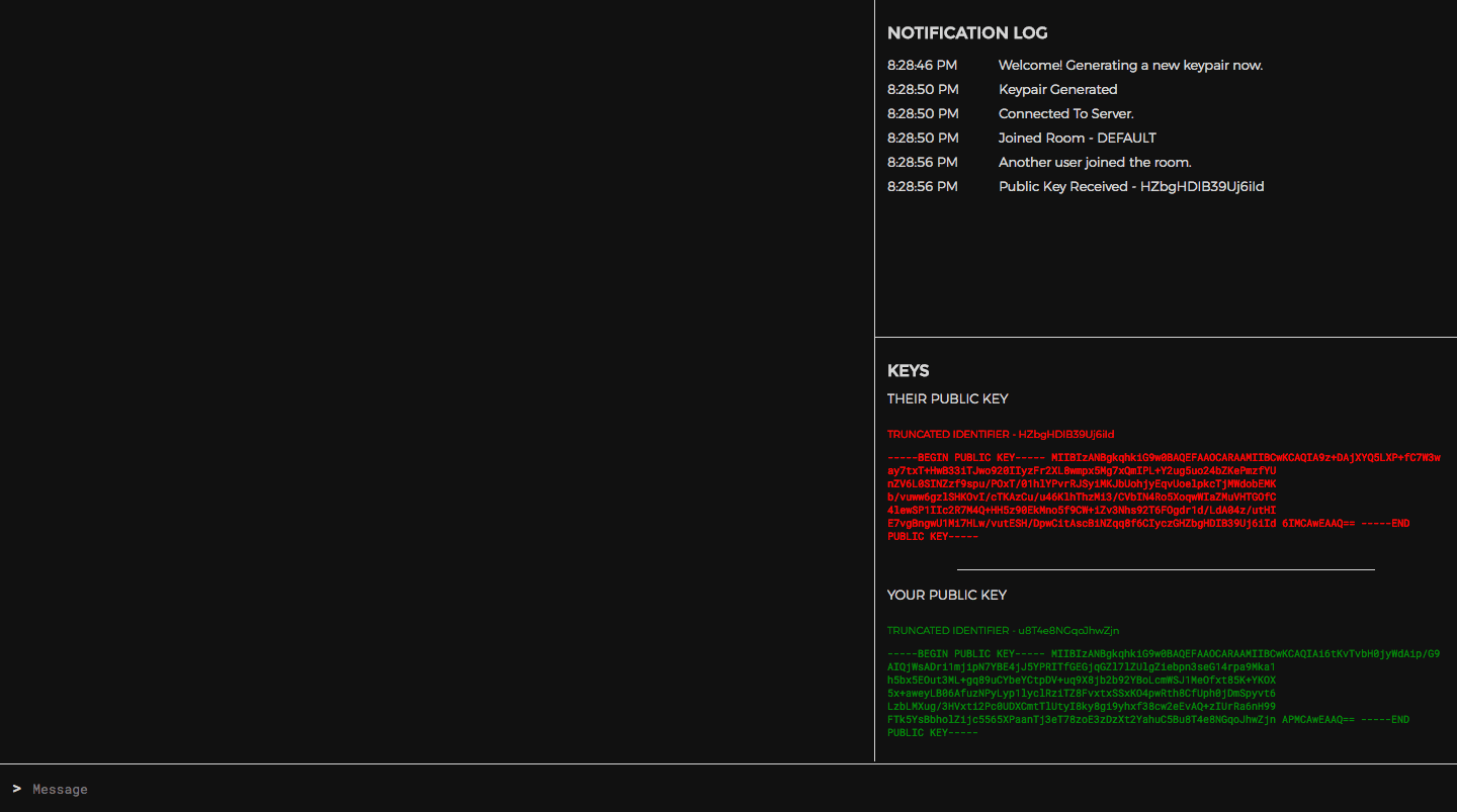
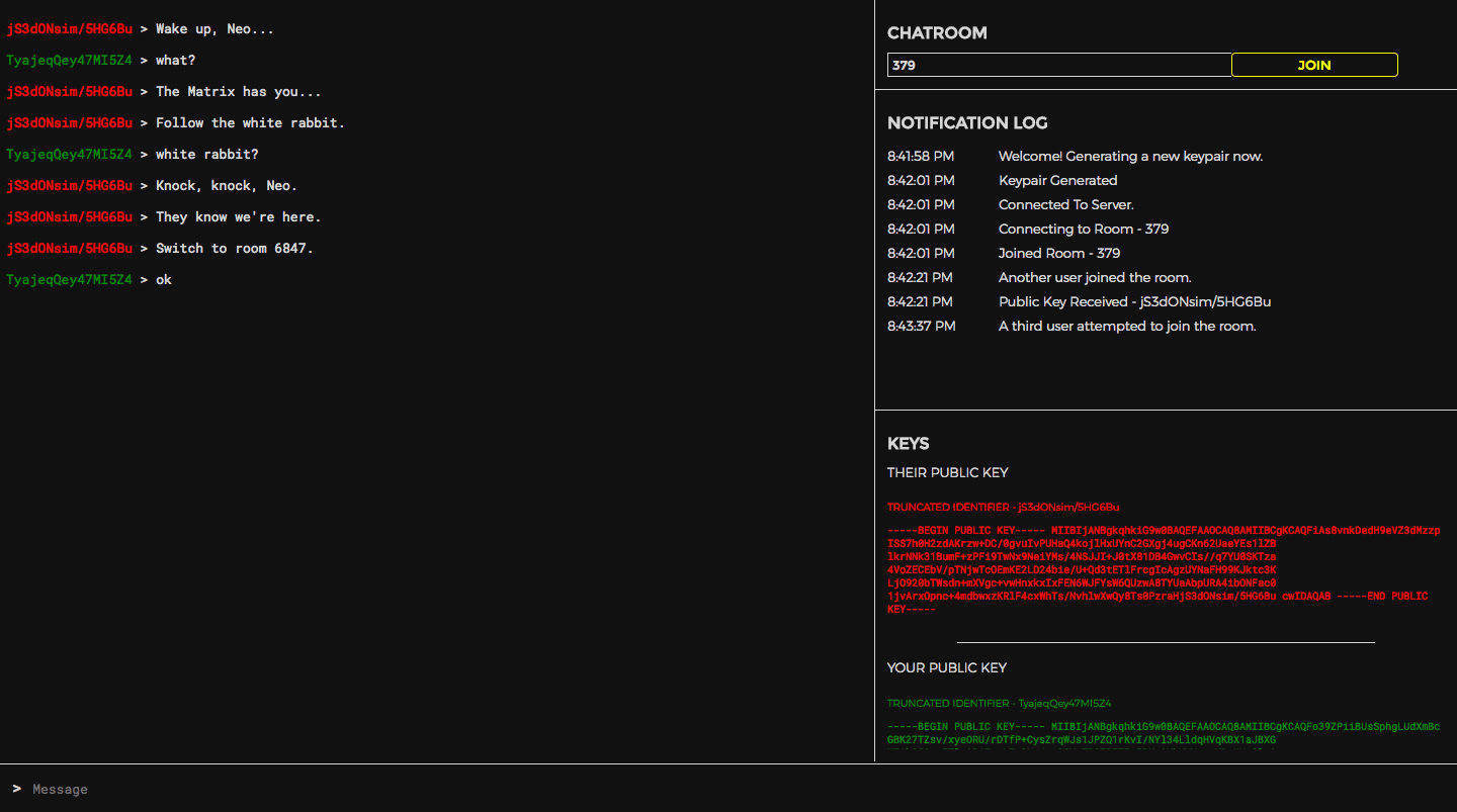
Finally, we'll add some HTML to display the two public keys.
Add the following to /public/index.html, directly below the <!-- Add Encryption Key UI Here --> comment.
<div class="divider"></div>
<div class="keys full-width">
  <h1>KEYS</h1>
  <h2>THEIR PUBLIC KEY</h2>
  <div class="key red" v-if="destinationPublicKey">
    <h3>TRUNCATED IDENTIFIER - {{ getKeySnippet(destinationPublicKey) }}</h3>
    <p>{{ destinationPublicKey }}</p>
  </div>
  <h2 v-else>Waiting for second user to join room...</h2>
  <div class="divider"></div>
  <h2>YOUR PUBLIC KEY</h2>
  <div class="key green" v-if="originPublicKey">
    <h3>TRUNCATED IDENTIFIER - {{ getKeySnippet(originPublicKey) }}</h3>
    <p>{{ originPublicKey }}</p>
  </div>
  <div class="keypair-loader full-width" v-else>
    <div class="center-x loader"></div>
    <h2 class="center-text">Generating Keypair...</h2>
  </div>
</div>
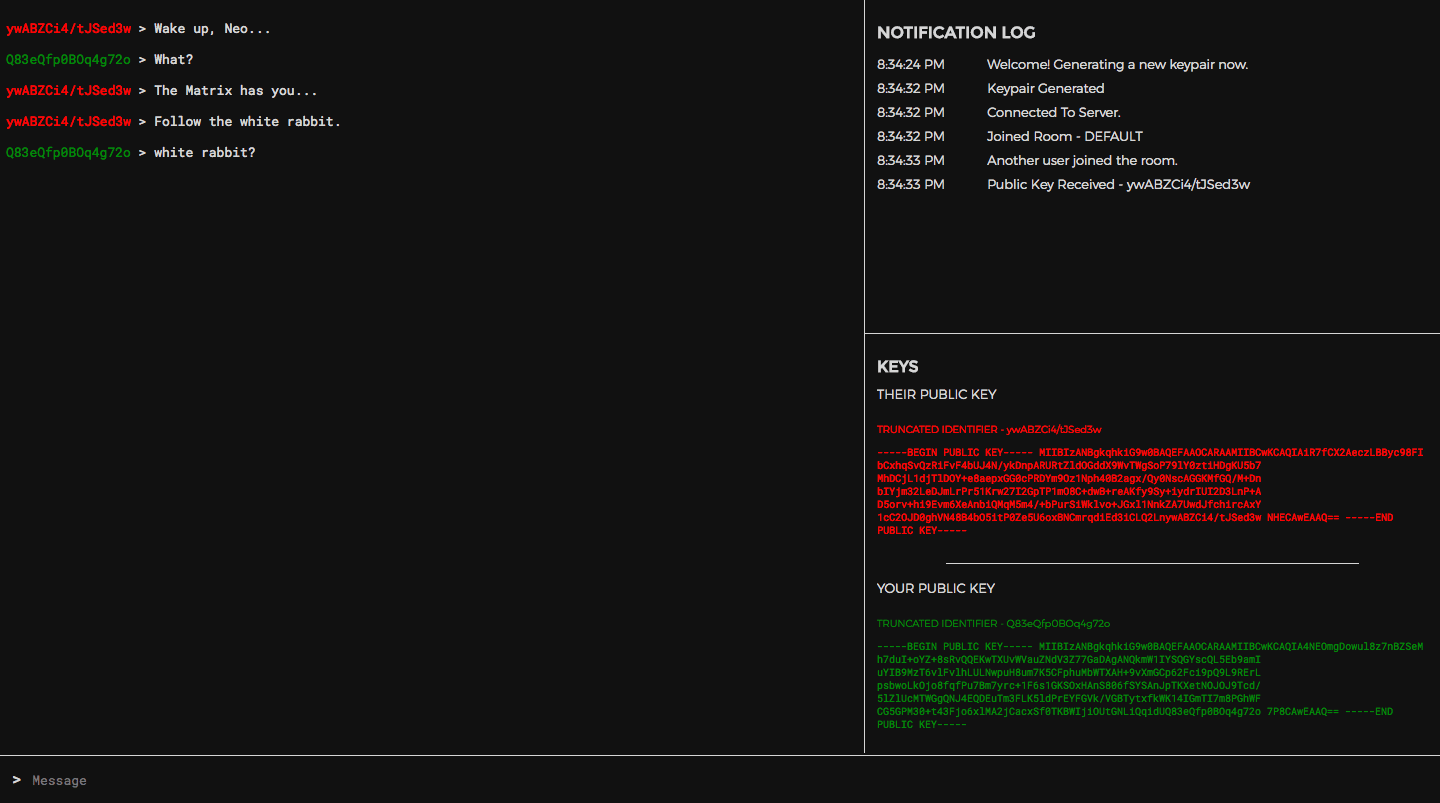
Try restarting the app and reloading https://localhost:3000. You should be able to simulate a successful key exchange by opening two browser tabs.
Having more than two pages with web app running will break the key-exchange. We'll fix this further down.
5 - Message Encryption
Now that the key-exchange is complete, encrypting and decrypting messages within the web app is rather straight-forward.
5.0 - Encrypt Message Before Sending
Replace the sendMessage function in /public/page.js with the following.
/** Encrypt and emit the current draft message */
async sendMessage () {
  // Don't send message if there is nothing to send
  if (!this.draft || this.draft === '') { return }
  // Use immutable.js to avoid unintended side-effects.
  let message = Immutable.Map({
    text: this.draft,
    recipient: this.destinationPublicKey,
    sender: this.originPublicKey
  })
  // Reset the UI input draft text
  this.draft = ''
  // Instantly add (unencrypted) message to local UI
  this.addMessage(message.toObject())
  if (this.destinationPublicKey) {
    // Encrypt message with the public key of the other user
    const encryptedText = await this.getWebWorkerResponse(
      'encrypt', [ message.get('text'), this.destinationPublicKey ])
    const encryptedMsg = message.set('text', encryptedText)
    // Emit the encrypted message
    this.socket.emit('MESSAGE', encryptedMsg.toObject())
  }
},
5.1 - Receive and Decrypt Message
Modify the client-side message listener in /public/page.js to decrypt the message once it is received.
// Decrypt and display message when received
this.socket.on('MESSAGE', async (message) => {
  // Only decrypt messages that were encrypted with the user's public key
  if (message.recipient === this.originPublicKey) {
    // Decrypt the message text in the webworker thread
    message.text = await this.getWebWorkerResponse('decrypt', message.text)
    // Instantly add (unencrypted) message to local UI
    this.addMessage(message)
  }
})
5.2 - Display Message List
Modify the message list UI in /public/index.html (inside the chat-container) to display the decrypted message and the abbreviated public key of the sender.
<div class="message full-width" v-for="message in messages">
  <p>
    <span v-bind:class="(message.sender == originPublicKey) ? 'green' : 'red'">{{ getKeySnippet(message.sender) }}</span>
    > {{ message.text }}
  </p>
</div>
5.3 - Try It Out
Try restarting the server and reloading the page at https://localhost:3000. The UI should look mostly unchanged from how it was before, besides displaying the public key snippet of whoever sent each message.
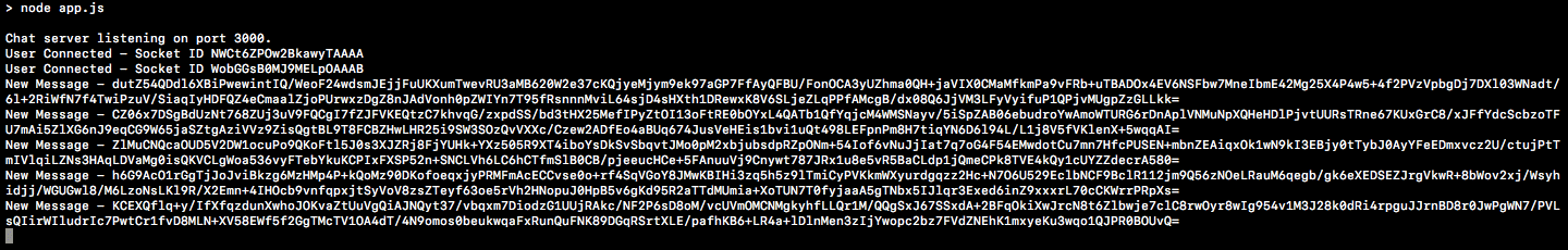
In command-line output, the messages are no longer readable - they now display as garbled encrypted text.
6 - Chatrooms
You may have noticed a massive flaw in the current app - if we open a third tab running the web app then the encryption system breaks. Asymmetric-encryption is designed to work in one-to-one scenarios; there's no way to encrypt the message once and have it be decryptable by two separate users.
This leaves us with two options -
- Encrypt and send a separate copy of the message to each user, if there is more than one.
- Restrict each chat room to only allow two users at a time.
Since this tutorial is already quite long, we'll be going with second, simpler option.
6.0 - Server-side Room Join Logic
In order to enforce this new 2-user limit, we'll modify the server-side socket JOIN listener in /app.js, at the top of socket connection listener block.
// Store the room that the socket is connected to
// If you need to scale the app horizontally, you'll need to store this variable in a persistent store such as Redis.
// For more info, see here: https://github.com/socketio/socket.io-redis
let currentRoom = null
/** Process a room join request. */
socket.on('JOIN', (roomName) => {
  // Get chatroom info
  let room = io.sockets.adapter.rooms[roomName]
  // Reject join request if room already has more than 1 connection
  if (room && room.length > 1) {
    // Notify user that their join request was rejected
    io.to(socket.id).emit('ROOM_FULL', null)
    // Notify room that someone tried to join
    socket.broadcast.to(roomName).emit('INTRUSION_ATTEMPT', null)
  } else {
    // Leave current room
    socket.leave(currentRoom)
    // Notify room that user has left
    socket.broadcast.to(currentRoom).emit('USER_DISCONNECTED', null)
    // Join new room
    currentRoom = roomName
    socket.join(currentRoom)
    // Notify user of room join success
    io.to(socket.id).emit('ROOM_JOINED', currentRoom)
    // Notify room that user has joined
    socket.broadcast.to(currentRoom).emit('NEW_CONNECTION', null)
  }
})
This modified socket logic will prevent a user from joining any room that already has two users.
6.1 - Join Room From The Client Side
Next, we'll modify our client-side joinRoom function in /public/page.js, in order to reset the state of the chat when switching rooms.
/** Join the specified chatroom */
joinRoom () {
  if (this.pendingRoom !== this.currentRoom && this.originPublicKey) {
    this.addNotification(`Connecting to Room - ${this.pendingRoom}`)
    // Reset room state variables
    this.messages = []
    this.destinationPublicKey = null
    // Emit room join request.
    this.socket.emit('JOIN', this.pendingRoom)
  }
},
6.2 - Add Notifications
Let's create two more client-side socket listeners (within the setupSocketListeners function in /public/page.js), to notify us whenever a join request is rejected.
// Notify user that the room they are attempting to join is full
this.socket.on('ROOM_FULL', () => {
  this.addNotification(`Cannot join ${this.pendingRoom}, room is full`)
  // Join a random room as a fallback
  this.pendingRoom = Math.floor(Math.random() * 1000)
  this.joinRoom()
})
// Notify room that someone attempted to join
this.socket.on('INTRUSION_ATTEMPT', () => {
  this.addNotification('A third user attempted to join the room.')
})
6.3 - Add Room Join UI
Finally, we'll add some HTML to provide an interface for the user to join a room of their choosing.
Add the following to /public/index.html below the <!-- Add Room UI Here --> comment.
<h1>CHATROOM</h1>
<div class="room-select">
  <input type="text" class="full-width" placeholder="Room Name" id="room-input" v-model="pendingRoom" @keyup.enter="joinRoom()">
  <input class="yellow-button full-width" type="submit" v-on:click="joinRoom()" value="JOIN">
</div>
<div class="divider"></div>
6.4 - Add Autoscroll
An annoying bug remaining in the app is that the notification and chat lists do not yet auto-scroll to display new messages.
In /public/page.js, add the following function to the methods block.
/** Autoscoll DOM element to bottom */
autoscroll (element) {
  if (element) { element.scrollTop = element.scrollHeight }
},
To auto-scroll the notification and message lists, we'll call autoscroll at the end of their respective add methods.
/** Add message to UI and scroll the view to display the new message. */
addMessage (message) {
  this.messages.push(message)
  this.autoscroll(this.$refs.chatContainer)
},
/** Append a notification message in the UI */
addNotification (message) {
  const timestamp = new Date().toLocaleTimeString()
  this.notifications.push({ message, timestamp })
  this.autoscroll(this.$refs.notificationContainer)
},
6.5 - Try it out
That was the last step! Try restarting the node app and reloading the page at localhost:3000. You should now be able to freely switch between rooms, and any attempt to join the same room from a third browser tab will be rejected.
7 - What next?
Congrats! You have just built a completely functional end-to-end encrypted messaging app.
Github Repository - https://github.com/triestpa/Open-Cryptochat
Live Preview - https://chat.patricktriest.com
Using this baseline source code you could deploy a private messaging app on your own servers. In order to coordinate which room to meet in, one slick option could be using a time-based pseudo-random number generator (such as Google Authenticator), with a shared seed between you and a second party (I've got a Javascript "Google Authenticator" clone tutorial in the works - stay tuned).
Further Improvements
There are lots of ways to build up the app from here:
- Group chats, by storing multiple public keys, and encrypting the message for each user individually.
- Multimedia messages, by encrypting a byte-array containing the media file.
- Import and export key pairs as local files.
- Sign messages with the private key for sender identity verification. This is a trade-off because it increases the difficulty of fabricating messages, but also undermines the goal of "deniable authentication" as outlined in the OTR messaging standard.
- Experiment with different encryption systems such as:
- AES - Symmetric encryption, with a shared secret between the users. This is the only publicly available algorithm that is in use by the NSA and US Military.
- ElGamal - Similar to RSA, but with smaller cyphertexts, faster decryption, and slower encryption. This is the core algorithm that is used in PGP.
- Implement a Diffie-Helman key exchange. This is a technique of using asymmetric encryption (such as ElGamal) to exchange a shared secret, such as a symmetric encryption key (for AES). Building this on top of our existing project and exchanging a new shared secret before each message is a good way to improve the security of the app (see Perfect Forward Security).
- Build an app for virtually any use-case where intermediate servers should never have unencrypted access to the transmitted data, such as password-managers and P2P (peer-to-peer) networks.
- Refactor the app for React Native, Ionic, Cordova, or Electron in order to provide a secure pre-built application bundle for mobile and/or desktop environments.
Feel free to comment below with questions, responses, and/or feedback on the tutorial.
Security Implications Of Browser Based Encryption
Please remember to be careful. The use of these protocols in a browser-based Javascript app is a great way to experiment and understand how they work in practice, but this app is not a suitable replacement for established, peer-reviewed encryption protocol implementations such as OpenSSL and GnuPG.
Client-side browser Javascript encryption is a controversial topic among security experts due to the vulnerabilities present in web application delivery versus pre-packaged software distributions that run outside the browser. Many of these issues can be mitigated by utilizing HTTPS to prevent man-in-the-middle resource injection attacks, and by avoiding persistent storage of unencrypted sensitive data within the browser, but it is important to stay aware of potential vulnerabilities in the web platform. ↩︎
Data Science, Politics, and Police

The intersection of science, politics, personal opinion, and social policy can be rather complex. This junction of ideas and disciplines is often rife with controversies, strongly held viewpoints, and agendas that are often more based on belief than on empirical evidence. Data science is particularly important in this area since it provides a methodology for examining the world in a pragmatic fact-first manner, and is capable of providing insight into some of the most important issues that we face today.
The recent high-profile police shootings of unarmed black men, such as Michael Brown (2014), Tamir Rice (2014), Anton Sterling (2016), and Philando Castile (2016), have triggered a divisive national dialog on the issue of racial bias in policing.
These shootings have spurred the growth of large social movements seeking to raise awareness of what is viewed as the systemic targeting of people-of-color by police forces across the country. On the other side of the political spectrum, many hold a view that the unbalanced targeting of non-white citizens is a myth created by the media based on a handful of extreme cases, and that these highly-publicized stories are not representative of the national norm.
In June 2017, a team of researchers at Stanford University collected and released an open-source data set of 60 million state police patrol stops from 20 states across the US. In this tutorial, we will walk through how to analyze and visualize this data using Python.
The source code and figures for this analysis can be found in the companion Github repository - https://github.com/triestpa/Police-Analysis-Python
To preview the completed IPython notebook, visit the page here.
This tutorial and analysis would not be possible without the work performed by The Stanford Open Policing Project. Much of the analysis performed in this tutorial is based on the work that has already performed by this team. A short tutorial for working with the data using the R programming language is provided on the official project website.
The Data
In the United States there are more than 50,000 traffic stops on a typical day. The potential number of data points for each stop is huge, from the demographics (age, race, gender) of the driver, to the location, time of day, stop reason, stop outcome, car model, and much more. Unfortunately, not every state makes this data available, and those that do often have different standards for which information is reported. Different counties and districts within each state can also be inconstant in how each traffic stop is recorded. The research team at Stanford has managed to gather traffic-stop data from twenty states, and has worked to regularize the reporting standards for 11 fields.
- Stop Date
- Stop Time
- Stop Location
- Driver Race
- Driver Gender
- Driver Age
- Stop Reason
- Search Conducted
- Search Type
- Contraband Found
- Stop Outcome
Most states do not have data available for every field, but there is enough overlap between the data sets to provide a solid foundation for some very interesting analysis.
0 - Getting Started
We'll start with analyzing the data set for Vermont. We're looking at Vermont first for a few reasons.
- The Vermont dataset is small enough to be very manageable and quick to operate on, with only 283,285 traffic stops (compared to the Texas data set, for instance, which contains almost 24 million records).
- There is not much missing data, as all eleven fields mentioned above are covered.
- Vermont is 94% white, but is also in a part of the country known for being very liberal (disclaimer - I grew up in the Boston area, and I've spent a quite a bit of time in Vermont). Many in this area consider this state to be very progressive and might like to believe that their state institutions are not as prone to systemic racism as the institutions in other parts of the country. It will be interesting to determine if the data validates this view.
0.0 - Download Datset
First, download the Vermont traffic stop data - https://stacks.stanford.edu/file/druid:py883nd2578/VT-clean.csv.gz
0.1 - Setup Project
Create a new directory for the project, say police-data-analysis, and move the downloaded file into a /data directory within the project.
0.2 - Optional: Create new virtualenv (or Anaconda) environment
If you want to keep your Python dependencies neat and separated between projects, now would be the time to create and activate a new environment for this analysis, using either virtualenv or Anaconda.
Here are some tutorials to help you get set up.
virtualenv - https://virtualenv.pypa.io/en/stable/
Anaconda - https://conda.io/docs/user-guide/install/index.html
0.3 - Install dependencies
We'll need to install a few Python packages to perform our analysis.
On the command line, run the following command to install the required libraries.
pip install numpy pandas matplotlib ipython jupyter
If you're using Anaconda, you can replace the
pipcommand here withconda. Also, depending on your installation, you might need to usepip3instead ofpipin order to install the Python 3 versions of the packages.
0.4 - Start Jupyter Notebook
Start a new local Jupyter notebook server from the command line.
jupyter notebook
Open your browser to the specified URL (probably localhost:8888, unless you have a special configuration) and create a new notebook.
I used Python 3.6 for writing this tutorial. If you want to use another Python version, that's fine, most of the code that we'll cover should work on any Python 2.x or 3.x distribution.
0.5 - Load Dependencies
In the first cell of the notebook, import our dependencies.
import pandas as pd
import numpy as np
import matplotlib.pyplot as plt
%matplotlib inline
figsize = (16,8)
We're also setting a shared variable figsize that we'll reuse later on in our data visualization logic.
0.6 - Load Dataset
In the next cell, load Vermont police stop data set into a Pandas dataframe.
df_vt = pd.read_csv('./data/VT-clean.csv.gz', compression='gzip', low_memory=False)
This command assumes that you are storing the data set in the
datadirectory of the project. If you are not, you can adjust the data file path accordingly.
1 - Vermont Data Exploration
Now begins the fun part.
1.0 - Preview the Available Data
We can get a quick preview of the first ten rows of the data set with the head() method.
df_vt.head()
| id | state | stop_date | stop_time | location_raw | county_name | county_fips | fine_grained_location | police_department | driver_gender | driver_age_raw | driver_age | driver_race_raw | driver_race | violation_raw | violation | search_conducted | search_type_raw | search_type | contraband_found | stop_outcome | is_arrested | officer_id | is_white | |
|---|---|---|---|---|---|---|---|---|---|---|---|---|---|---|---|---|---|---|---|---|---|---|---|---|
| 0 | VT-2010-00001 | VT | 2010-07-01 | 00:10 | East Montpelier | Washington County | 50023.0 | COUNTY RD | MIDDLESEX VSP | M | 22.0 | 22.0 | White | White | Moving Violation | Moving violation | False | No Search Conducted | N/A | False | Citation | False | -1.562157e+09 | True |
| 3 | VT-2010-00004 | VT | 2010-07-01 | 00:11 | Whiting | Addison County | 50001.0 | N MAIN ST | NEW HAVEN VSP | F | 18.0 | 18.0 | White | White | Moving Violation | Moving violation | False | No Search Conducted | N/A | False | Arrest for Violation | True | -3.126844e+08 | True |
| 4 | VT-2010-00005 | VT | 2010-07-01 | 00:35 | Hardwick | Caledonia County | 50005.0 | i91 nb mm 62 | ROYALTON VSP | M | 18.0 | 18.0 | White | White | Moving Violation | Moving violation | False | No Search Conducted | N/A | False | Written Warning | False | 9.225661e+08 | True |
| 5 | VT-2010-00006 | VT | 2010-07-01 | 00:44 | Hardwick | Caledonia County | 50005.0 | 64000 I 91 N; MM64 I 91 N | ROYALTON VSP | F | 20.0 | 20.0 | White | White | Vehicle Equipment | Equipment | False | No Search Conducted | N/A | False | Written Warning | False | -6.032327e+08 | True |
| 8 | VT-2010-00009 | VT | 2010-07-01 | 01:10 | Rochester | Windsor County | 50027.0 | 36000 I 91 S; MM36 I 91 S | ROCKINGHAM VSP | M | 24.0 | 24.0 | Black | Black | Moving Violation | Moving violation | False | No Search Conducted | N/A | False | Written Warning | False | 2.939526e+08 | False |
We can also list the available fields by reading the columns property.
df_vt.columns
Index(['id', 'state', 'stop_date', 'stop_time', 'location_raw', 'county_name',
       'county_fips', 'fine_grained_location', 'police_department',
       'driver_gender', 'driver_age_raw', 'driver_age', 'driver_race_raw',
       'driver_race', 'violation_raw', 'violation', 'search_conducted',
       'search_type_raw', 'search_type', 'contraband_found', 'stop_outcome',
       'is_arrested', 'officer_id'],
      dtype='object')
1.1 - Drop Missing Values
Let's do a quick count of each column to determine how consistently populated the data is.
df_vt.count()
id                       283285
state                    283285
stop_date                283285
stop_time                283285
location_raw             282591
county_name              282580
county_fips              282580
fine_grained_location    282938
police_department        283285
driver_gender            281573
driver_age_raw           282114
driver_age               281999
driver_race_raw          279301
driver_race              278468
violation_raw            281107
violation                281107
search_conducted         283285
search_type_raw          281045
search_type                3419
contraband_found         283251
stop_outcome             280960
is_arrested              283285
officer_id               283273
dtype: int64
We can see that most columns have similar numbers of values besides search_type, which is not present for most of the rows, likely because most stops do not result in a search.
For our analysis, it will be best to have the exact same number of values for each field. We'll go ahead now and make sure that every single cell has a value.
# Fill missing search type values with placeholder
df_vt['search_type'].fillna('N/A', inplace=True)
# Drop rows with missing values
df_vt.dropna(inplace=True)
df_vt.count()
When we count the values again, we'll see that each column has the exact same number of entries.
id                       273181
state                    273181
stop_date                273181
stop_time                273181
location_raw             273181
county_name              273181
county_fips              273181
fine_grained_location    273181
police_department        273181
driver_gender            273181
driver_age_raw           273181
driver_age               273181
driver_race_raw          273181
driver_race              273181
violation_raw            273181
violation                273181
search_conducted         273181
search_type_raw          273181
search_type              273181
contraband_found         273181
stop_outcome             273181
is_arrested              273181
officer_id               273181
dtype: int64
1.2 - Stops By County
Let's get a list of all counties in the data set, along with how many traffic stops happened in each.
df_vt['county_name'].value_counts()
Windham County       37715
Windsor County       36464
Chittenden County    24815
Orange County        24679
Washington County    24633
Rutland County       22885
Addison County       22813
Bennington County    22250
Franklin County      19715
Caledonia County     16505
Orleans County       10344
Lamoille County       8604
Essex County          1239
Grand Isle County      520
Name: county_name, dtype: int64
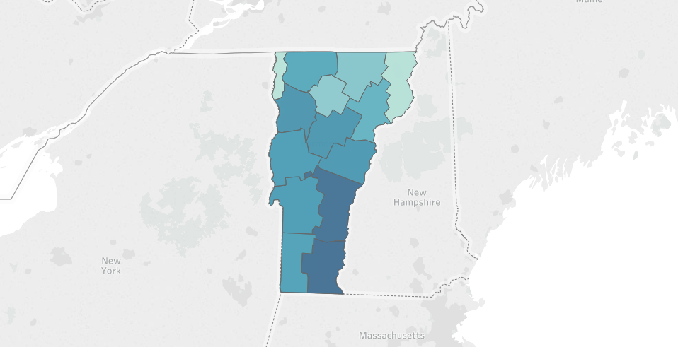
If you're familiar with Vermont's geography, you'll notice that the police stops seem to be more concentrated in counties in the southern-half of the state. The southern-half of the state is also where much of the cross-state traffic flows in transit to and from New Hampshire, Massachusetts, and New York. Since the traffic stop data is from the state troopers, this interstate highway traffic could potentially explain why we see more traffic stops in these counties.
Here's a quick map generated with Tableau to visualize this regional distribution.
1.3 - Violations
We can also check out the distribution of traffic stop reasons.
df_vt['violation'].value_counts()
Moving violation      212100
Equipment              50600
Other                   9768
DUI                      711
Other (non-mapped)         2
Name: violation, dtype: int64
Unsurprisingly, the top reason for a traffic stop is Moving Violation (speeding, reckless driving, etc.), followed by Equipment (faulty lights, illegal modifications, etc.).
By using the violation_raw fields as reference, we can see that the Other category includes "Investigatory Stop" (the police have reason to suspect that the driver of the vehicle has committed a crime) and "Externally Generated Stop" (possibly as a result of a 911 call, or a referral from municipal police departments).
DUI ("driving under the influence", i.e. drunk driving) is surprisingly the least prevalent, with only 711 total recorded stops for this reason over the five year period (2010-2015) that the dataset covers. This seems low, since Vermont had 2,647 DUI arrests in 2015, so I suspect that a large proportion of these arrests were performed by municipal police departments, and/or began with a Moving Violation stop, instead of a more specific DUI stop.
1.4 - Outcomes
We can also examine the traffic stop outcomes.
df_vt['stop_outcome'].value_counts()
Written Warning         166488
Citation                103401
Arrest for Violation      3206
Warrant Arrest              76
Verbal Warning              10
Name: stop_outcome, dtype: int64
A majority of stops result in a written warning - which goes on the record but carries no direct penalty. A bit over 1/3 of the stops result in a citation (commonly known as a ticket), which comes with a direct fine and can carry other negative side-effects such as raising a driver's auto insurance premiums.
The decision to give a warning or a citation is often at the discretion of the police officer, so this could be a good source for studying bias.
1.5 - Stops By Gender
Let's break down the traffic stops by gender.
df_vt['driver_gender'].value_counts()
M    179678
F    101895
Name: driver_gender, dtype: int64
We can see that approximately 36% of the stops are of women drivers, and 64% are of men.
1.6 - Stops By Race
Let's also examine the distribution by race.
df_vt['driver_race'].value_counts()
White       266216
Black         5741
Asian         3607
Hispanic      2625
Other          279
Name: driver_race, dtype: int64
Most traffic stops are of white drivers, which is to be expected since Vermont is around 94% white (making it the 2nd-least diverse state in the nation, behind Maine). Since white drivers make up approximately 94% of the traffic stops, there's no obvious bias here for pulling over non-white drivers vs white drivers. Using the same methodology, however, we can also see that while black drivers make up roughly 2% of all traffic stops, only 1.3% of Vermont's population is black.
Let's keep on analyzing the data to see what else we can learn.
1.7 - Police Stop Frequency by Race and Age
It would be interesting to visualize how the frequency of police stops breaks down by both race and age.
fig, ax = plt.subplots()
ax.set_xlim(15, 70)
for race in df_vt['driver_race'].unique():
    s = df_vt[df_vt['driver_race'] == race]['driver_age']
    s.plot.kde(ax=ax, label=race)
ax.legend()
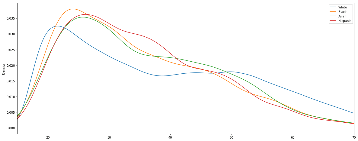
We can see that young drivers in their late teens and early twenties are the most likely to be pulled over. Between ages 25 and 35, the stop rate of each demographic drops off quickly. As far as the racial comparison goes, the most interesting disparity is that for white drivers between the ages of 35 and 50 the pull-over rate stays mostly flat, whereas for other races it continues to drop steadily.
2 - Violation and Outcome Analysis
Now that we've got a feel for the dataset, we can start getting into some more advanced analysis.
One interesting topic that we touched on earlier is the fact that the decision to penalize a driver with a ticket or a citation is often at the discretion of the police officer. With this in mind, let's see if there are any discernable patterns in driver demographics and stop outcome.
2.0 - Analysis Helper Function
In order to assist in this analysis, we'll define a helper function to aggregate a few important statistics from our dataset.
citations_per_warning- The ratio of citations to warnings. A higher number signifies a greater likelihood of being ticketed instead of getting off with a warning.arrest_rate- The percentage of stops that end in an arrest.
def compute_outcome_stats(df):
    """Compute statistics regarding the relative quanties of arrests, warnings, and citations"""
    n_total = len(df)
    n_warnings = len(df[df['stop_outcome'] == 'Written Warning'])
    n_citations = len(df[df['stop_outcome'] == 'Citation'])
    n_arrests = len(df[df['stop_outcome'] == 'Arrest for Violation'])
    citations_per_warning = n_citations / n_warnings
    arrest_rate = n_arrests / n_total
    return(pd.Series(data = {
        'n_total': n_total,
        'n_warnings': n_warnings,
        'n_citations': n_citations,
        'n_arrests': n_arrests,
        'citations_per_warning': citations_per_warning,
        'arrest_rate': arrest_rate
    }))
Let's test out this helper function by applying it to the entire dataframe.
compute_outcome_stats(df_vt)
arrest_rate                   0.011721
citations_per_warning         0.620751
n_arrests                  3199.000000
n_citations              103270.000000
n_total                  272918.000000
n_warnings               166363.000000
dtype: float64
In the above result, we can see that about 1.17% of traffic stops result in an arrest, and there are on-average 0.62 citations (tickets) issued per warning. This data passes the sanity check, but it's too coarse to provide many interesting insights. Let's dig deeper.
2.1 - Breakdown By Gender
Using our helper function, along with the Pandas dataframe groupby method, we can easily compare these stats for male and female drivers.
df_vt.groupby('driver_gender').apply(compute_outcome_stats)
| arrest_rate | citations_per_warning | n_arrests | n_citations | n_total | n_warnings | |
|---|---|---|---|---|---|---|
| driver_gender | ||||||
| F | 0.007038 | 0.548033 | 697.0 | 34805.0 | 99036.0 | 63509.0 |
| M | 0.014389 | 0.665652 | 2502.0 | 68465.0 | 173882.0 | 102854.0 |
This is a simple example of the common split-apply-combine technique. We'll be building on this pattern for the remainder of the tutorial, so make sure that you understand how this comparison table is generated before continuing.
We can see here that men are, on average, twice as likely to be arrested during a traffic stop, and are also slightly more likely to be given a citation than women. It is, of course, not clear from the data whether this is indicative of any bias by the police officers, or if it reflects that men are being pulled over for more serious offenses than women on average.
2.2 - Breakdown By Race
Let's now compute the same comparison, grouping by race.
df_vt.groupby('driver_race').apply(compute_outcome_stats)
| arrest_rate | citations_per_warning | n_arrests | n_citations | n_total | n_warnings | |
|---|---|---|---|---|---|---|
| driver_race | ||||||
| Asian | 0.006384 | 1.002339 | 22.0 | 1714.0 | 3446.0 | 1710.0 |
| Black | 0.019925 | 0.802379 | 111.0 | 2428.0 | 5571.0 | 3026.0 |
| Hispanic | 0.016393 | 0.865827 | 42.0 | 1168.0 | 2562.0 | 1349.0 |
| White | 0.011571 | 0.611188 | 3024.0 | 97960.0 | 261339.0 | 160278.0 |
Ok, this is interesting. We can see that Asian drivers are arrested at the lowest rate, but receive tickets at the highest rate (roughly 1 ticket per warning). Black and Hispanic drivers are both arrested at a higher rate and ticketed at a higher rate than white drivers.
Let's visualize these results.
race_agg = df_vt.groupby(['driver_race']).apply(compute_outcome_stats)
fig, axes = plt.subplots(nrows=2, ncols=1, figsize=figsize)
race_agg['citations_per_warning'].plot.barh(ax=axes[0], figsize=figsize, title="Citation Rate By Race")
race_agg['arrest_rate'].plot.barh(ax=axes[1], figsize=figsize, title='Arrest Rate By Race')
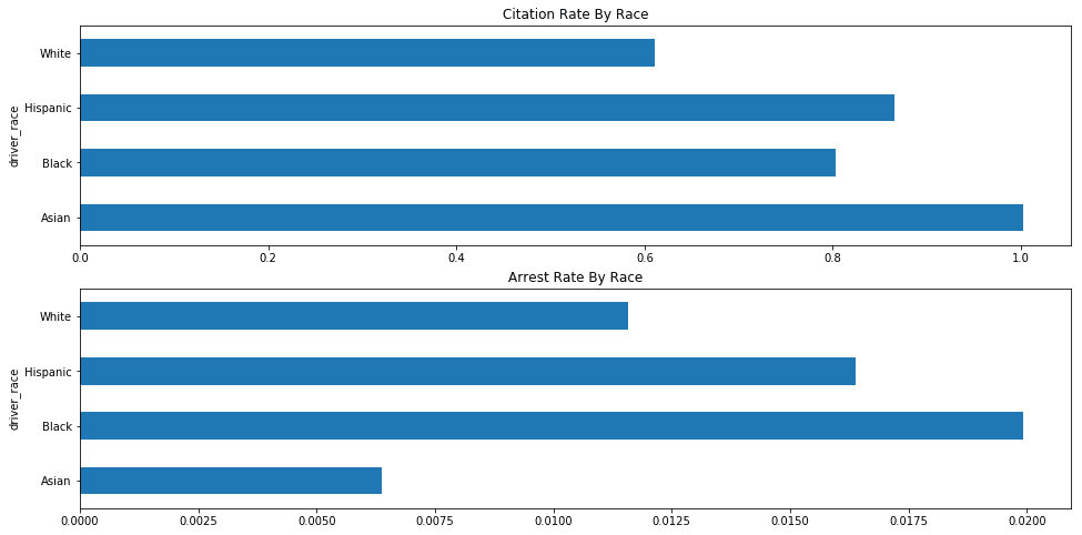
2.3 - Group By Outcome and Violation
We'll deepen our analysis by grouping each statistic by the violation that triggered the traffic stop.
df_vt.groupby(['driver_race','violation']).apply(compute_outcome_stats)
| arrest_rate | citations_per_warning | n_arrests | n_citations | n_total | n_warnings | ||
|---|---|---|---|---|---|---|---|
| driver_race | violation | ||||||
| Asian | DUI | 0.200000 | 0.333333 | 2.0 | 2.0 | 10.0 | 6.0 |
| Equipment | 0.006270 | 0.132143 | 2.0 | 37.0 | 319.0 | 280.0 | |
| Moving violation | 0.005563 | 1.183190 | 17.0 | 1647.0 | 3056.0 | 1392.0 | |
| Other | 0.016393 | 0.875000 | 1.0 | 28.0 | 61.0 | 32.0 | |
| Black | DUI | 0.200000 | 0.142857 | 2.0 | 1.0 | 10.0 | 7.0 |
| Equipment | 0.029181 | 0.220651 | 26.0 | 156.0 | 891.0 | 707.0 | |
| Moving violation | 0.016052 | 0.942385 | 71.0 | 2110.0 | 4423.0 | 2239.0 | |
| Other | 0.048583 | 2.205479 | 12.0 | 161.0 | 247.0 | 73.0 | |
| Hispanic | DUI | 0.200000 | 3.000000 | 2.0 | 6.0 | 10.0 | 2.0 |
| Equipment | 0.023560 | 0.187898 | 9.0 | 59.0 | 382.0 | 314.0 | |
| Moving violation | 0.012422 | 1.058824 | 26.0 | 1062.0 | 2093.0 | 1003.0 | |
| Other | 0.064935 | 1.366667 | 5.0 | 41.0 | 77.0 | 30.0 | |
| White | DUI | 0.192364 | 0.455026 | 131.0 | 172.0 | 681.0 | 378.0 |
| Equipment | 0.012233 | 0.190486 | 599.0 | 7736.0 | 48965.0 | 40612.0 | |
| Moving violation | 0.008635 | 0.732720 | 1747.0 | 84797.0 | 202321.0 | 115729.0 | |
| Other | 0.058378 | 1.476672 | 547.0 | 5254.0 | 9370.0 | 3558.0 | |
| Other (non-mapped) | 0.000000 | 1.000000 | 0.0 | 1.0 | 2.0 | 1.0 |
Ok, well this table looks interesting, but it's rather large and visually overwhelming. Let's trim down that dataset in order to retrieve a more focused subset of information.
# Create new column to represent whether the driver is white
df_vt['is_white'] = df_vt['driver_race'] == 'White'
# Remove violation with too few data points
df_vt_filtered = df_vt[~df_vt['violation'].isin(['Other (non-mapped)', 'DUI'])]
We're generating a new column to represent whether or not the driver is white. We are also generating a filtered version of the dataframe that strips out the two violation types with the fewest datapoints.
We not assigning the filtered dataframe to
df_vtsince we'll want to keep using the complete unfiltered dataset in the next sections.
Let's redo our race + violation aggregation now, using our filtered dataset.
df_vt_filtered.groupby(['is_white','violation']).apply(compute_outcome_stats)
| arrest_rate | citations_per_warning | n_arrests | n_citations | n_total | n_warnings | ||
|---|---|---|---|---|---|---|---|
| is_white | violation | ||||||
| False | Equipment | 0.023241 | 0.193697 | 37.0 | 252.0 | 1592.0 | 1301.0 |
| Moving violation | 0.011910 | 1.039922 | 114.0 | 4819.0 | 9572.0 | 4634.0 | |
| Other | 0.046753 | 1.703704 | 18.0 | 230.0 | 385.0 | 135.0 | |
| True | Equipment | 0.012233 | 0.190486 | 599.0 | 7736.0 | 48965.0 | 40612.0 |
| Moving violation | 0.008635 | 0.732720 | 1747.0 | 84797.0 | 202321.0 | 115729.0 | |
| Other | 0.058378 | 1.476672 | 547.0 | 5254.0 | 9370.0 | 3558.0 |
Ok great, this is much easier to read.
In the above table, we can see that non-white drivers are more likely to be arrested during a stop that was initiated due to an equipment or moving violation, but white drivers are more likely to be arrested for a traffic stop resulting from "Other" reasons. Non-white drivers are more likely than white drivers to be given tickets for each violation.
2.4 - Visualize Stop Outcome and Violation Results
Let's generate a bar chart now in order to visualize this data broken down by race.
race_stats = df_vt_filtered.groupby(['violation', 'driver_race']).apply(compute_outcome_stats).unstack()
fig, axes = plt.subplots(nrows=1, ncols=2, figsize=figsize)
race_stats.plot.bar(y='arrest_rate', ax=axes[0], title='Arrest Rate By Race and Violation')
race_stats.plot.bar(y='citations_per_warning', ax=axes[1], title='Citations Per Warning By Race and Violation')
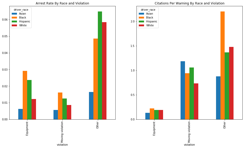
We can see in these charts that Hispanic and Black drivers are generally arrested at a higher rate than white drivers (with the exception of the rather ambiguous "Other" category). and that Black drivers are more likely, across the board, to be issued a citation than white drivers. Asian drivers are arrested at very low rates, and their citation rates are highly variable.
These results are compelling, and are suggestive of potential racial bias, but they are too inconsistent across violation types to provide any definitive answers. Let's dig deeper to see what else we can find.
3 - Search Outcome Analysis
Two of the more interesting fields available to us are search_conducted and contraband_found.
In the analysis by the "Stanford Open Policing Project", they use these two fields to perform what is known as an "outcome test".
On the project website, the "outcome test" is summarized clearly.
In the 1950s, the Nobel prize-winning economist Gary Becker proposed an elegant method to test for bias in search decisions: the outcome test.
Becker proposed looking at search outcomes. If officers don’t discriminate, he argued, they should find contraband — like illegal drugs or weapons — on searched minorities at the same rate as on searched whites. If searches of minorities turn up contraband at lower rates than searches of whites, the outcome test suggests officers are applying a double standard, searching minorities on the basis of less evidence."
Findings, Stanford Open Policing Project
The authors of the project also make the point that only using the "hit rate", or the rate of searches where contraband is found, can be misleading. For this reason, we'll also need to use the "search rate" in our analysis - the rate at which a traffic stop results in a search.
We'll now use the available data to perform our own outcome test, in order to determine whether minorities in Vermont are routinely searched on the basis of less evidence than white drivers.
3.0 Compute Search Rate and Hit Rate
We'll define a new function to compute the search rate and hit rate for the traffic stops in our dataframe.
- Search Rate - The rate at which a traffic stop results in a search. A search rate of
0.20would signify that out of 100 traffic stops, 20 resulted in a search. - Hit Rate - The rate at which contraband is found in a search. A hit rate of
0.80would signify that out of 100 searches, 80 searches resulted in contraband (drugs, unregistered weapons, etc.) being found.
def compute_search_stats(df):
    """Compute the search rate and hit rate"""
    search_conducted = df['search_conducted']
    contraband_found = df['contraband_found']
    n_stops     = len(search_conducted)
    n_searches  = sum(search_conducted)
    n_hits      = sum(contraband_found)
    # Filter out counties with too few stops
    if (n_stops) < 50:
        search_rate = None
    else:
        search_rate = n_searches / n_stops
    # Filter out counties with too few searches
    if (n_searches) < 5:
        hit_rate = None
    else:
        hit_rate = n_hits / n_searches
    return(pd.Series(data = {
        'n_stops': n_stops,
        'n_searches': n_searches,
        'n_hits': n_hits,
        'search_rate': search_rate,
        'hit_rate': hit_rate
    }))
3.1 - Compute Search Stats For Entire Dataset
We can test our new function to determine the search rate and hit rate for the entire state.
compute_search_stats(df_vt)
hit_rate            0.796865
n_hits           2593.000000
n_searches       3254.000000
n_stops        272918.000000
search_rate         0.011923
dtype: float64
Here we can see that each traffic stop had a 1.2% change of resulting in a search, and each search had an 80% chance of yielding contraband.
3.2 - Compare Search Stats By Driver Gender
Using the Pandas groupby method, we can compute how the search stats differ by gender.
df_vt.groupby('driver_gender').apply(compute_search_stats)
| hit_rate | n_hits | n_searches | n_stops | search_rate | |
|---|---|---|---|---|---|
| driver_gender | |||||
| F | 0.789392 | 506.0 | 641.0 | 99036.0 | 0.006472 |
| M | 0.798699 | 2087.0 | 2613.0 | 173882.0 | 0.015027 |
We can see here that men are three times as likely to be searched as women, and that 80% of searches for both genders resulted in contraband being found. The data shows that men are searched and caught with contraband more often than women, but it is unclear whether there is any gender discrimination in deciding who to search since the hit rate is equal.
3.3 - Compare Search Stats By Age
We can split the dataset into age buckets and perform the same analysis.
age_groups = pd.cut(df_vt["driver_age"], np.arange(15, 70, 5))
df_vt.groupby(age_groups).apply(compute_search_stats)
| hit_rate | n_hits | n_searches | n_stops | search_rate | |
|---|---|---|---|---|---|
| driver_age | |||||
| (15, 20] | 0.847988 | 569.0 | 671.0 | 27418.0 | 0.024473 |
| (20, 25] | 0.838000 | 838.0 | 1000.0 | 43275.0 | 0.023108 |
| (25, 30] | 0.788462 | 492.0 | 624.0 | 34759.0 | 0.017952 |
| (30, 35] | 0.766756 | 286.0 | 373.0 | 27746.0 | 0.013443 |
| (35, 40] | 0.742991 | 159.0 | 214.0 | 23203.0 | 0.009223 |
| (40, 45] | 0.692913 | 88.0 | 127.0 | 24055.0 | 0.005280 |
| (45, 50] | 0.575472 | 61.0 | 106.0 | 24103.0 | 0.004398 |
| (50, 55] | 0.706667 | 53.0 | 75.0 | 22517.0 | 0.003331 |
| (55, 60] | 0.833333 | 30.0 | 36.0 | 17502.0 | 0.002057 |
| (60, 65] | 0.500000 | 6.0 | 12.0 | 12514.0 | 0.000959 |
We can see here that the search rate steadily declines as drivers get older, and that the hit rate also declines rapidly for older drivers.
3.4 - Compare Search Stats By Race
Now for the most interesting part - comparing search data by race.
df_vt.groupby('driver_race').apply(compute_search_stats)
| hit_rate | n_hits | n_searches | n_stops | search_rate | |
|---|---|---|---|---|---|
| driver_race | |||||
| Asian | 0.785714 | 22.0 | 28.0 | 3446.0 | 0.008125 |
| Black | 0.686620 | 195.0 | 284.0 | 5571.0 | 0.050978 |
| Hispanic | 0.644231 | 67.0 | 104.0 | 2562.0 | 0.040593 |
| White | 0.813601 | 2309.0 | 2838.0 | 261339.0 | 0.010859 |
Black and Hispanic drivers are searched at much higher rates than White drivers (5% and 4% of traffic stops respectively, versus 1% for white drivers), but the searches of these drivers only yield contraband 60-70% of the time, compared to 80% of the time for White drivers.
Let's rephrase these results.
Black drivers are 500% more likely to be searched than white drivers during a traffic stop, but are 13% less likely to be caught with contraband in the event of a search.
Hispanic drivers are 400% more likely to be searched than white drivers during a traffic stop, but are 17% less likely to be caught with contraband in the event of a search.
3.5 - Compare Search Stats By Race and Location
Let's add in location as another factor. It's possible that some counties (such as those with larger towns or with interstate highways where opioid trafficking is prevalent) have a much higher search rate / lower hit rates for both white and non-white drivers, but also have greater racial diversity, leading to distortion in the overall stats. By controlling for location, we can determine if this is the case.
We'll define three new helper functions to generate the visualizations.
def generate_comparison_scatter(df, ax, state, race, field, color):
    """Generate scatter plot comparing field for white drivers with minority drivers"""
    race_location_agg = df.groupby(['county_fips','driver_race']).apply(compute_search_stats).reset_index().dropna()
    race_location_agg = race_location_agg.pivot(index='county_fips', columns='driver_race', values=field)
    ax = race_location_agg.plot.scatter(ax=ax, x='White', y=race, s=150, label=race, color=color)
    return ax
def format_scatter_chart(ax, state, field):
    """Format and label to scatter chart"""
    ax.set_xlabel('{} - White'.format(field))
    ax.set_ylabel('{} - Non-White'.format(field, race))
    ax.set_title("{} By County - {}".format(field, state))
    lim = max(ax.get_xlim()[1], ax.get_ylim()[1])
    ax.set_xlim(0, lim)
    ax.set_ylim(0, lim)
    diag_line, = ax.plot(ax.get_xlim(), ax.get_ylim(), ls="--", c=".3")
    ax.legend()
    return ax
def generate_comparison_scatters(df, state):
    """Generate scatter plots comparing search rates of white drivers with black and hispanic drivers"""
    fig, axes = plt.subplots(nrows=1, ncols=2, figsize=figsize)
    generate_comparison_scatter(df, axes[0], state, 'Black', 'search_rate', 'red')
    generate_comparison_scatter(df, axes[0], state, 'Hispanic', 'search_rate', 'orange')
    generate_comparison_scatter(df, axes[0], state, 'Asian', 'search_rate', 'green')
    format_scatter_chart(axes[0], state, 'Search Rate')
    generate_comparison_scatter(df, axes[1], state, 'Black', 'hit_rate', 'red')
    generate_comparison_scatter(df, axes[1], state, 'Hispanic', 'hit_rate', 'orange')
    generate_comparison_scatter(df, axes[1], state, 'Asian', 'hit_rate', 'green')
    format_scatter_chart(axes[1], state, 'Hit Rate')
    return fig
We can now generate the scatter plots using the generate_comparison_scatters function.
generate_comparison_scatters(df_vt, 'VT')
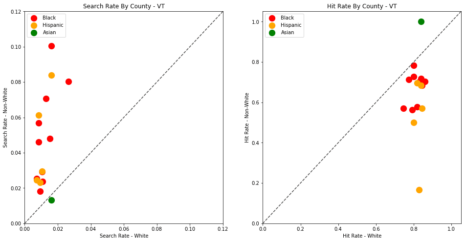
The plots above are comparing search_rate (left) and hit_rate (right) for minority drivers compared with white drivers in each county. If all of the dots (each of which represents the stats for a single county and race) followed the diagonal center line, the implication would be that white drivers and non-white drivers are searched at the exact same rate with the exact same standard of evidence.
Unfortunately, this is not the case. In the above charts, we can see that, for every county, the search rate is higher for Black and Hispanic drivers even though the hit rate is lower.
Let's define one more visualization helper function, to show all of these results on a single scatter plot.
def generate_county_search_stats_scatter(df, state):
    """Generate a scatter plot of search rate vs. hit rate by race and county"""
    race_location_agg = df.groupby(['county_fips','driver_race']).apply(compute_search_stats)
    colors = ['blue','orange','red', 'green']
    fig, ax = plt.subplots(figsize=figsize)
    for c, frame in race_location_agg.groupby(level='driver_race'):
        ax.scatter(x=frame['hit_rate'], y=frame['search_rate'], s=150, label=c, color=colors.pop())
    ax.legend(loc='upper center', bbox_to_anchor=(0.5, 1.2), ncol=4, fancybox=True)
    ax.set_xlabel('Hit Rate')
    ax.set_ylabel('Search Rate')
    ax.set_title("Search Stats By County and Race - {}".format(state))
    return fig
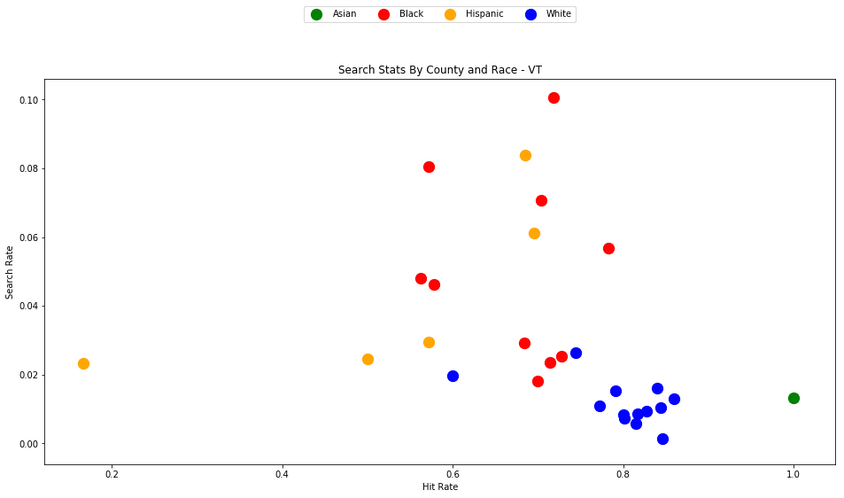
generate_county_search_stats_scatter(df_vt, "VT")
As the old idiom goes - a picture is worth a thousand words. The above chart is one of those pictures - and the name of the picture is "Systemic Racism".
The search rates and hit rates for white drivers in most counties are consistently clustered around 80% and 1% respectively. We can see, however, that nearly every county searches Black and Hispanic drivers at a higher rate, and that these searches uniformly have a lower hit rate than those on White drivers.
This state-wide pattern of a higher search rate combined with a lower hit rate suggests that a lower standard of evidence is used when deciding to search Black and Hispanic drivers compared to when searching White drivers.
You might notice that only one county is represented by Asian drivers - this is due to the lack of data for searches of Asian drivers in other counties.
4 - Analyzing Other States
Vermont is a great state to test out our analysis on, but the dataset size is relatively small. Let's now perform the same analysis on other states to determine if this pattern persists across state lines.
4.0 - Massachusetts
First we'll generate the analysis for my home state, Massachusetts. This time we'll have more data to work with - roughly 3.4 million traffic stops.
Download the dataset to your project's /data directory - https://stacks.stanford.edu/file/druid:py883nd2578/MA-clean.csv.gz
We've developed a solid reusable formula for reading and visualizing each state's dataset, so let's wrap the entire recipe in a new helper function.
fields = ['county_fips', 'driver_race', 'search_conducted', 'contraband_found']
types = {
    'contraband_found': bool,
    'county_fips': float,
    'driver_race': object,
    'search_conducted': bool
}
def analyze_state_data(state):
    df = pd.read_csv('./data/{}-clean.csv.gz'.format(state), compression='gzip', low_memory=True, dtype=types, usecols=fields)
    df.dropna(inplace=True)
    df = df[df['driver_race'] != 'Other']
    generate_comparison_scatters(df, state)
    generate_county_search_stats_scatter(df, state)
    return df.groupby('driver_race').apply(compute_search_stats)
We're making a few optimizations here in order to make the analysis a bit more streamlined and computationally efficient. By only reading the four columns that we're interested in, and by specifying the datatypes ahead of time, we'll be able to read larger datasets into memory more quickly.
analyze_state_data('MA')
The first output is a statewide table of search rate and hit rate by race.
| hit_rate | n_hits | n_searches | n_stops | search_rate | |
|---|---|---|---|---|---|
| driver_race | |||||
| Asian | 0.331169 | 357.0 | 1078.0 | 101942.0 | 0.010575 |
| Black | 0.487150 | 4170.0 | 8560.0 | 350498.0 | 0.024422 |
| Hispanic | 0.449502 | 5007.0 | 11139.0 | 337782.0 | 0.032977 |
| White | 0.523037 | 18220.0 | 34835.0 | 2527393.0 | 0.013783 |
We can see here again that Black and Hispanic drivers are searched at significantly higher rates than white drivers. The differences in hit rates are not as extreme as in Vermont, but they are still noticeably lower for Black and Hispanic drivers than for White drivers. Asian drivers, interestingly, are the least likely to be searched and also the least likely to have contraband if they are searched.
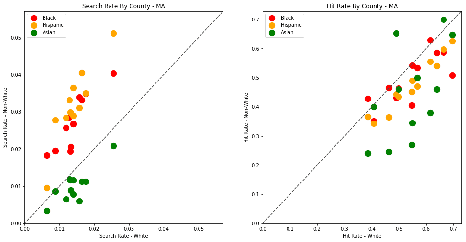
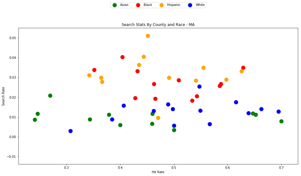
If we compare the stats for MA to VT, we'll also notice that police in MA seem to use a much lower standard of evidence when searching a vehicle, with their searches averaging around a 50% hit rate, compared to 80% in VT.
The trend here is much less obvious than in Vermont, but it is still clear that traffic stops of Black and Hispanic drivers are more likely to result in a search, despite the fact the searches of White drivers are more likely to result in contraband being found.
4.1 - Wisconsin & Connecticut
Wisconsin and Connecticut have been named as some of the worst states in America for racial disparities. Let's see how their police stats stack up.
Again, you'll need to download the Wisconsin and Connecticut dataset to your project's /data directory.
- Wisconsin: https://stacks.stanford.edu/file/druid:py883nd2578/WI-clean.csv.gz
- Connecticut: https://stacks.stanford.edu/file/druid:py883nd2578/WI-clean.csv.gz
We can call our analyze_state_data function for Wisconsin once the dataset has been downloaded.
analyze_state_data('WI')
| hit_rate | n_hits | n_searches | n_stops | search_rate | |
|---|---|---|---|---|---|
| driver_race | |||||
| Asian | 0.470817 | 121.0 | 257.0 | 24577.0 | 0.010457 |
| Black | 0.477574 | 1299.0 | 2720.0 | 56050.0 | 0.048528 |
| Hispanic | 0.415741 | 449.0 | 1080.0 | 35210.0 | 0.030673 |
| White | 0.526300 | 5103.0 | 9696.0 | 778227.0 | 0.012459 |
The trends here are starting to look familiar. White drivers in Wisconsin are much less likely to be searched than non-white drivers (aside from Asians, who tend to be searched at around the same rates as whites). Searches of non-white drivers are, again, less likely to yield contraband than searches on white drivers.
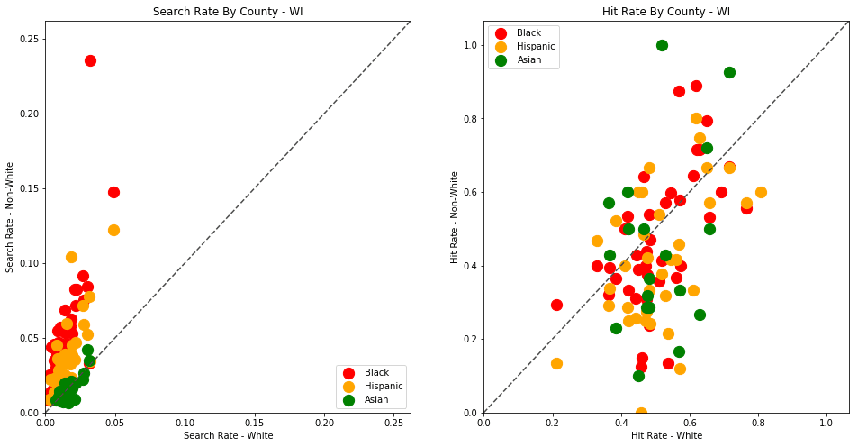
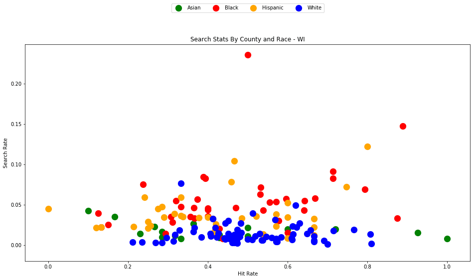
We can see here, yet again, that the standard of evidence for searching Black and Hispanic drivers is lower in virtually every county than for White drivers. In one outlying county, almost 25% (!) of traffic stops for Black drivers resulted in a search, even though only half of those searches yielded contraband.
Let's do the same analysis for Connecticut
analyze_state_data('CT')
| hit_rate | n_hits | n_searches | n_stops | search_rate | |
|---|---|---|---|---|---|
| driver_race | |||||
| Asian | 0.384615 | 10.0 | 26.0 | 5949.0 | 0.004370 |
| Black | 0.284072 | 346.0 | 1218.0 | 37460.0 | 0.032515 |
| Hispanic | 0.291925 | 282.0 | 966.0 | 31154.0 | 0.031007 |
| White | 0.379344 | 1179.0 | 3108.0 | 242314.0 | 0.012826 |
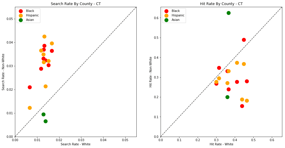
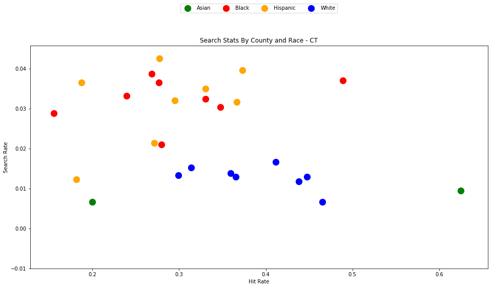
Again, the pattern persists.
4.2 - Arizona
We can generate each result rather quickly for each state (with available data), once we've downloaded each dataset.
analyze_state_data('AZ')
| hit_rate | n_hits | n_searches | n_stops | search_rate | |
|---|---|---|---|---|---|
| driver_race | |||||
| Asian | 0.196664 | 224.0 | 1139.0 | 48177.0 | 0.023642 |
| Black | 0.255548 | 2188.0 | 8562.0 | 116795.0 | 0.073308 |
| Hispanic | 0.160930 | 5943.0 | 36929.0 | 501619.0 | 0.073620 |
| White | 0.242564 | 9288.0 | 38291.0 | 1212652.0 | 0.031576 |
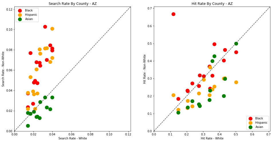
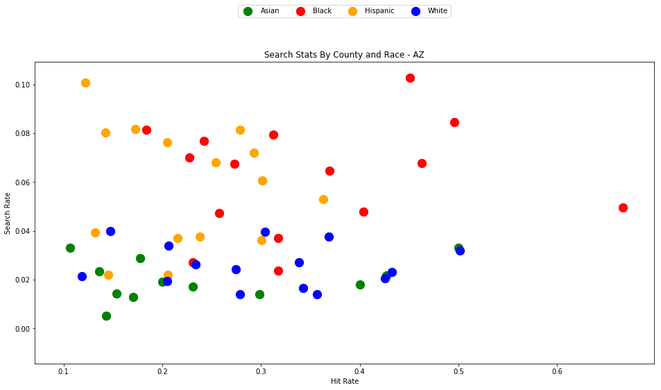
4.3 - Colorado
analyze_state_data('CO')
| hit_rate | n_hits | n_searches | n_stops | search_rate | |
|---|---|---|---|---|---|
| driver_race | |||||
| Asian | 0.537634 | 50.0 | 93.0 | 32471.0 | 0.002864 |
| Black | 0.481283 | 270.0 | 561.0 | 71965.0 | 0.007795 |
| Hispanic | 0.450454 | 1041.0 | 2311.0 | 308499.0 | 0.007491 |
| White | 0.651388 | 3638.0 | 5585.0 | 1767804.0 | 0.003159 |
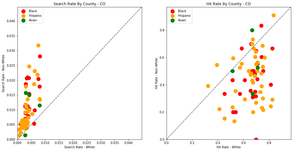
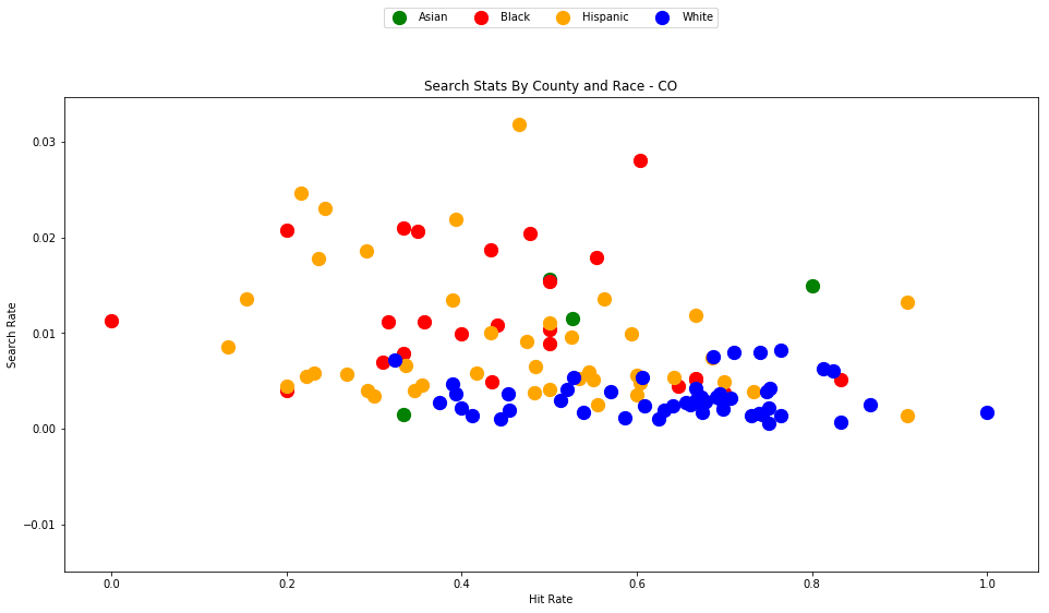
4.4 - Washington
analyze_state_data('WA')
| hit_rate | n_hits | n_searches | n_stops | search_rate | |
|---|---|---|---|---|---|
| driver_race | |||||
| Asian | 0.087143 | 608.0 | 6977.0 | 352063.0 | 0.019817 |
| Black | 0.130799 | 1717.0 | 13127.0 | 254577.0 | 0.051564 |
| Hispanic | 0.103366 | 2128.0 | 20587.0 | 502254.0 | 0.040989 |
| White | 0.156008 | 15768.0 | 101072.0 | 4279273.0 | 0.023619 |
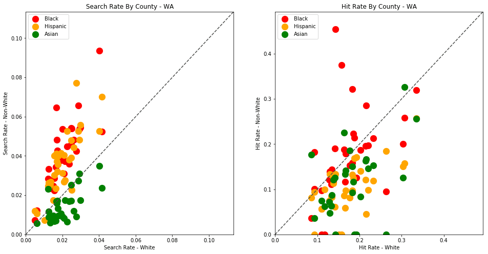
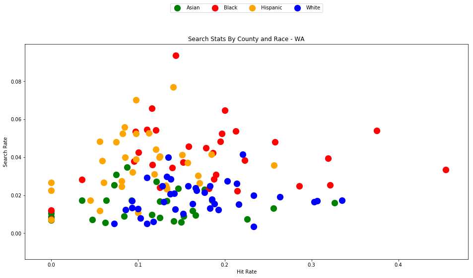
4.5 - North Carolina
analyze_state_data('NC')
| hit_rate | n_hits | n_searches | n_stops | search_rate | |
|---|---|---|---|---|---|
| driver_race | |||||
| Asian | 0.104377 | 31.0 | 297.0 | 46287.0 | 0.006416 |
| Black | 0.182489 | 1955.0 | 10713.0 | 1222533.0 | 0.008763 |
| Hispanic | 0.119330 | 776.0 | 6503.0 | 368878.0 | 0.017629 |
| White | 0.153850 | 3387.0 | 22015.0 | 3146302.0 | 0.006997 |
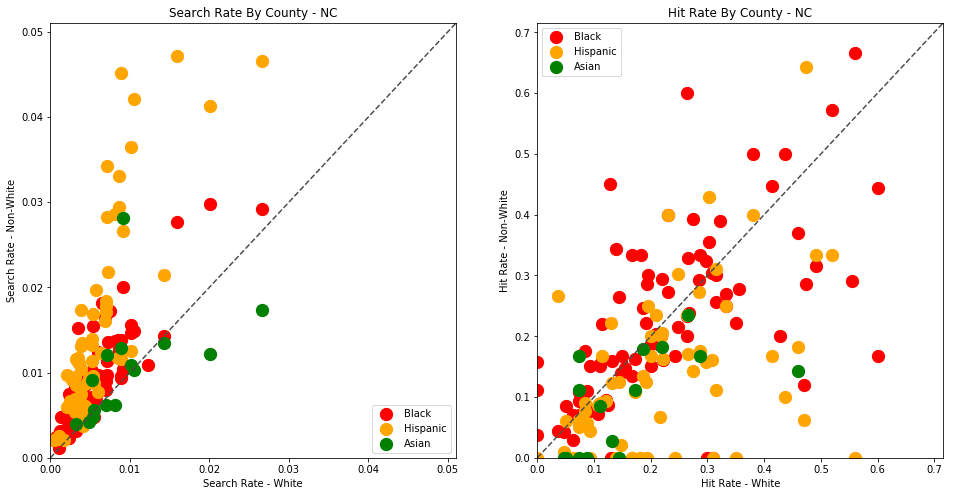
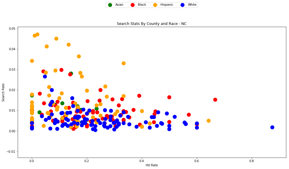
4.6 - Texas
You might want to let this one run while you go fix yourself a cup of coffee or tea. At almost 24 million traffic stops, the Texas dataset takes a rather long time to process.
analyze_state_data('TX')
| hit_rate | n_hits | n_searches | n_stops | search_rate | |
|---|---|---|---|---|---|
| driver_race | |||||
| Asian | 0.289271 | 976.0 | 3374.0 | 349105.0 | 0.009665 |
| Black | 0.345983 | 27588.0 | 79738.0 | 2300427.0 | 0.034662 |
| Hispanic | 0.219449 | 37080.0 | 168969.0 | 6525365.0 | 0.025894 |
| White | 0.335098 | 83157.0 | 248157.0 | 13576726.0 | 0.018278 |
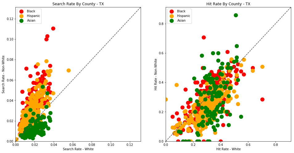
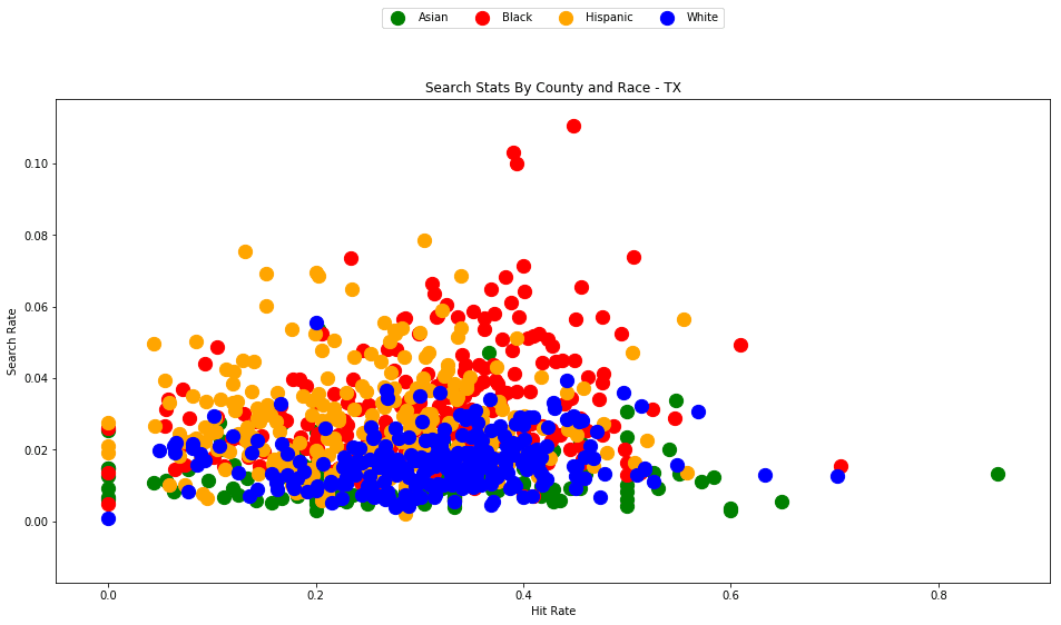
4.7 - Even more data visualizations
I highly recommend that you visit the Stanford Open Policing Project results page for more visualizations of this data. Here you can browse the search outcome results for all available states, and explore additional analysis that the researchers have performed such as stop rate by race (using county population demographics data) as well as the effects of recreational marijuana legalization on search rates.
5 - What next?
Do these results imply that all police officers are overtly racist? No.
Do they show that Black and Hispanic drivers are searched much more frequently than white drivers, often with a lower standard of evidence? Yes.
What we are observing here appears to be a pattern of systemic racism. The racial disparities revealed in this analysis are a reflection of an entrenched mistrust of certain minorities in the United States. The data and accompanying analysis are indicative of social trends that are certainly not limited to police officers. Racial discrimination is present at all levels of society from retail stores to the tech industry to academia.
We are able to empirically identify these trends only because state police deparments (and the Open Policing team at Stanford) have made this data available to the public; no similar datasets exist for most other professions and industries. Releasing datasets about these issues is commendable (but sadly still somewhat uncommon, especially in the private sector) and will help to further identify where these disparities exist, and to influence policies in order to provide a fair, effective way to counteract these biases.
To see the full official analysis for all 20 available states, check out the official findings paper here - https://5harad.com/papers/traffic-stops.pdf.
I hope that this tutorial has provided the tools you might need to take this analysis further. There's a lot more that you can do with the data than what we've covered here.
- Analyze police stops for your home state and county (if the data is available). If the data is not available, submit a formal request to your local representatives and institutions that the data be made public.
- Combine your analysis with US census data on the demographic, social, and economic stats about each county.
- Create a web app to display the county trends on an interactive map.
- Build a mobile app to warn drivers when they're entering an area that appears to be more distrusting of drivers of a certain race.
- Open-source your own analysis, spread your findings, seek out peer review, maybe even write an explanatory blog post.
The source code and figures for this analysis can be found in the companion Github repository - https://github.com/triestpa/Police-Analysis-Python
To view the completed IPython notebook, visit the page here.
The code for this project is 100% open source (MIT license), so feel free to use it however you see fit in your own projects.
As always, please feel free to comment below with any questions, comments, or criticisms.

Regular Expressions (Regex): One of the most powerful, widely applicable, and sometimes intimidating techniques in software engineering. From validating email addresses to performing complex code refactors, regular expressions have a wide range of uses and are an essential entry in any software engineer's toolbox.
What is a regular expression?
A regular expression (or regex, or regexp) is a way to describe complex search patterns using sequences of characters.
The complexity of the specialized regex syntax, however, can make these expressions somewhat inaccessible. For instance, here is a basic regex that describes any time in the 24-hour HH/MM format.
\b([01]?[0-9]|2[0-3]):([0-5]\d)\b
If this looks complex to you now, don't worry, by the time we finish the tutorial understanding this expression will be trivial.
Learn once, write anywhere
Regular expressions can be used in virtually any programming language. A knowledge of regex is very useful for validating user input, interacting with the Unix shell, searching/refactoring code in your favorite text editor, performing database text searches, and lots more.
In this tutorial, I'll attempt to give an provide an approachable introduction to regex syntax and usage in a variety of scenarios, languages, and environments.
This web application is my favorite tool for building, testing, and debugging regular expressions. I highly recommend that you use it to test out the expressions that we'll cover in this tutorial.
The source code for the examples in this tutorial can be found at the Github repository here - https://github.com/triestpa/You-Should-Learn-Regex
0 - Match Any Number Line
We'll start with a very simple example - Match any line that only contains numbers.
^[0-9]+$
Let's walk through this piece-by-piece.
^- Signifies the start of a line.[0-9]- Matches any digit between 0 and 9+- Matches one or more instance of the preceding expression.$- Signifies the end of the line.
We could re-write this regex in pseudo-English as [start of line][one or more digits][end of line].
Pretty simple right?
We could replace
[0-9]with\d, which will do the same thing (match any digit).
The great thing about this expression (and regular expressions in general) is that it can be used, without much modification, in any programing language.
To demonstrate we'll now quickly go through how to perform this simple regex search on a text file using 16 of the most popular programming languages.
We can use the following input file (test.txt) as an example.
1234
abcde
12db2
5362
1
Each script will read the test.txt file, search it using our regular expression, and print the result ('1234', '5362', '1') to the console.
Language Examples
0.0 - Javascript / Node.js / Typescript
const fs = require('fs')
const testFile = fs.readFileSync('test.txt', 'utf8')
const regex = /^([0-9]+)$/gm
let results = testFile.match(regex)
console.log(results)
0.1 - Python
import re
with open('test.txt', 'r') as f:
  test_string = f.read()
  regex = re.compile(r'^([0-9]+)$', re.MULTILINE)
  result = regex.findall(test_string)
  print(result)
0.2 - R
fileLines <- readLines("test.txt")
results <- grep("^[0-9]+$", fileLines, value = TRUE)
print (results)
0.3 - Ruby
File.open("test.txt", "rb") do |f|
    test_str = f.read
    re = /^[0-9]+$/m
    test_str.scan(re) do |match|
        puts match.to_s
    end
end
0.4 - Haskell
import Text.Regex.PCRE
main = do
  fileContents <- readFile "test.txt"
  let stringResult = fileContents =~ "^[0-9]+$" :: AllTextMatches [] String
  print (getAllTextMatches stringResult)
0.5 - Perl
open my $fh, '<', 'test.txt' or die "Unable to open file $!";
read $fh, my $file_content, -s $fh;
close $fh;
my $regex = qr/^([0-9]+)$/mp;
my @matches = $file_content =~ /$regex/g;
print join(',', @matches);
0.6 - PHP
<?php
$myfile = fopen("test.txt", "r") or die("Unable to open file.");
$test_str = fread($myfile,filesize("test.txt"));
fclose($myfile);
$re = '/^[0-9]+$/m';
preg_match_all($re, $test_str, $matches, PREG_SET_ORDER, 0);
var_dump($matches);
?>
0.7 - Go
package main
import (
    "fmt"
    "io/ioutil"
    "regexp"
)
func main() {
    testFile, err := ioutil.ReadFile("test.txt")
    if err != nil { fmt.Print(err) }
    testString := string(testFile)
    var re = regexp.MustCompile(`(?m)^([0-9]+)$`)
    var results = re.FindAllString(testString, -1)
    fmt.Println(results)
}
0.8 - Java
import java.util.regex.Matcher;
import java.util.regex.Pattern;
import java.io.IOException;
import java.nio.file.Files;
import java.nio.file.Paths;
import java.util.ArrayList;
class FileRegexExample {
  public static void main(String[] args) {
    try {
      String content = new String(Files.readAllBytes(Paths.get("test.txt")));
      Pattern pattern = Pattern.compile("^[0-9]+$", Pattern.MULTILINE);
      Matcher matcher = pattern.matcher(content);
      ArrayList<String> matchList = new ArrayList<String>();
      while (matcher.find()) {
        matchList.add(matcher.group());
      }
      System.out.println(matchList);
    } catch (IOException e) {
      e.printStackTrace();
    }
  }
}
0.9 - Kotlin
import java.io.File
import kotlin.text.Regex
import kotlin.text.RegexOption
val file = File("test.txt")
val content:String = file.readText()
val regex = Regex("^[0-9]+$", RegexOption.MULTILINE)
val results = regex.findAll(content).map{ result -> result.value }.toList()
println(results)
0.10 - Scala
import scala.io.Source
import scala.util.matching.Regex
object FileRegexExample {
  def main(args: Array[String]) {
    val fileContents = Source.fromFile("test.txt").getLines.mkString("\n")
    val pattern = "(?m)^[0-9]+$".r
    val results = (pattern findAllIn fileContents).mkString(",")
    println(results)
  }
}
0.11 - Swift
import Cocoa
do {
    let fileText = try String(contentsOfFile: "test.txt", encoding: String.Encoding.utf8)
    let regex = try! NSRegularExpression(pattern: "^[0-9]+$", options: [ .anchorsMatchLines ])
    let results = regex.matches(in: fileText, options: [], range: NSRange(location: 0, length: fileText.characters.count))
    let matches = results.map { String(fileText[Range($0.range, in: fileText)!]) }
    print(matches)
} catch {
    print(error)
}
0.12 - Rust
extern crate regex;
use std::fs::File;
use std::io::prelude::*;
use regex::Regex;
fn main() {
  let mut f = File::open("test.txt").expect("file not found");
  let mut test_str = String::new();
  f.read_to_string(&mut test_str).expect("something went wrong reading the file");
  let regex = match Regex::new(r"(?m)^([0-9]+)$") {
    Ok(r) => r,
    Err(e) => {
      println!("Could not compile regex: {}", e);
      return;
    }
  };
  let result = regex.find_iter(&test_str);
  for mat in result {
    println!("{}", &test_str[mat.start()..mat.end()]);
  }
}
0.13 - C#
using System;
using System.IO;
using System.Text;
using System.Text.RegularExpressions;
using System.Linq;
namespace RegexExample
{
    class FileRegexExample
    {
        static void Main()
        {
            string text = File.ReadAllText(@"./test.txt", Encoding.UTF8);
            Regex regex = new Regex("^[0-9]+$", RegexOptions.Multiline);
            MatchCollection mc = regex.Matches(text);
            var matches = mc.OfType<Match>().Select(m => m.Value).ToArray();
            Console.WriteLine(string.Join(" ", matches));
        }
    }
}
0.14 - C++
#include <string>
#include <fstream>
#include <iostream>
#include <sstream>
#include <regex>
using namespace std;
int main () {
  ifstream t("test.txt");
  stringstream buffer;
  buffer << t.rdbuf();
  string testString = buffer.str();
  regex numberLineRegex("(^|\n)([0-9]+)($|\n)");
  sregex_iterator it(testString.begin(), testString.end(), numberLineRegex);
  sregex_iterator it_end;
  while(it != it_end) {
    cout << it -> str();
    ++it;
  }
}
0.15 - Bash
#!bin/bash
grep -E '^[0-9]+$' test.txt
Writing out the same operation in sixteen languages is a fun exercise, but we'll be mostly sticking with Javascript and Python (along with a bit of Bash at the end) for the rest of the tutorial since these languages (in my opinion) tend to yield the clearest and most readable implementations.
1 - Year Matching
Let's go through another simple example - matching any valid year in the 20th or 21st centuries.
\b(19|20)\d{2}\b
We're starting and ending this regex with \b instead of ^ and $. \b represents a word boundary, or a space between two words. This will allow us to match years within the text blocks (instead of on their own lines), which is very useful for searching through, say, paragraph text.
\b- Word boundary(19|20)- Matches either '19' or '20' using the OR (|) operand.\d{2}- Two digits, same as[0-9]{2}\b- Word boundary
Note that
\bdiffers from\s, the code for a whitespace character.\bsearches for a place where a word character is not followed or preceded by another word-character, so it is searching for the absence of a word character, whereas\sis searching explicitly for a space character.\bis especially appropriate for cases where we want to match a specific sequence/word, but not the whitespace before or after it.
1.0 - Real-World Example - Count Year Occurrences
We can use this expression in a Python script to find how many times each year in the 20th or 21st century is mentioned in a historical Wikipedia article.
import re
import urllib.request
import operator
# Download wiki page
url = "https://en.wikipedia.org/wiki/Diplomatic_history_of_World_War_II"
html = urllib.request.urlopen(url).read()
# Find all mentioned years in the 20th or 21st century
regex = r"\b(?:19|20)\d{2}\b"
matches = re.findall(regex, str(html))
# Form a dict of the number of occurrences of each year
year_counts = dict((year, matches.count(year)) for year in set(matches))
# Print the dict sorted in descending order
for year in sorted(year_counts, key=year_counts.get, reverse=True):
  print(year, year_counts[year])
The above script will print each year, along the number of times it is mentioned.
1941 137
1943 80
1940 76
1945 73
1939 71
...
2 - Time Matching
Now we'll define a regex expression to match any time in the 24-hour format (MM:HH, such as 16:59).
\b([01]?[0-9]|2[0-3]):([0-5]\d)\b
\b- Word boundary[01]- 0 or 1?- Signifies that the preceding pattern is optional.[0-9]- any number between 0 and 9|-ORoperand2[0-3]- 2, followed by any number between 0 and 3 (i.e. 20-23):- Matches the:character[0-5]- Any number between 0 and 5\d- Any number between 0 and 9 (same as[0-9])\b- Word boundary
2.0 - Capture Groups
You might have noticed something new in the above pattern - we're wrapping the hour and minute capture segments in parenthesis ( ... ). This allows us to define each part of the pattern as a capture group.
Capture groups allow us individually extract, transform, and rearrange pieces of each matched pattern.
2.1 - Real-World Example - Time Parsing
For example, in the above 24-hour pattern, we've defined two capture groups - one for the hour and one for the minute.
We can extract these capture groups easily.
Here's how we could use Javascript to parse a 24-hour formatted time into hours and minutes.
const regex = /\b([01]?[0-9]|2[0-3]):([0-5]\d)/
const str = `The current time is 16:24`
const result = regex.exec(str)
console.log(`The current hour is ${result[1]}`)
console.log(`The current minute is ${result[2]}`)
The zeroth capture group is always the entire matched expression.
The above script will produce the following output.
The current hour is 16
The current minute is 24
As an extra exercise, you could try modifying this script to convert 24-hour times to 12-hour (am/pm) times.
3 - Date Matching
Now let's match a DAY/MONTH/YEAR style date pattern.
\b(0?[1-9]|[12]\d|3[01])([\/\-])(0?[1-9]|1[012])\2(\d{4})
This one is a bit longer, but it should look pretty similar to what we've covered already.
(0?[1-9]|[12]\d|3[01])- Match any number between 1 and 31 (with an optional preceding zero)([\/\-])- Match the seperator/or-(0?[1-9]|1[012])- Match any number between 1 and 12\2- Matches the second capture group (the seperator)\d{4}- Match any 4 digit number (0000 - 9999)
The only new concept here is that we're using \2 to match the second capture group, which is the divider (/ or -). This enables us to avoid repeating our pattern matching specification, and will also require that the dividers are consistent (if the first divider is /, then the second must be as well).
3.0 - Capture Group Substitution
Using capture groups, we can dynamically reorganize and transform our string input.
The standard way to refer to capture groups is to use the $ or \ symbol, along with the index of the capture group.
3.1 - Real-World Example - Date Format Transformation
Let's imagine that we were tasked with converting a collection of documents from using the international date format style (DAY/MONTH/YEAR) to the American style (MONTH/DAY/YEAR)
We could use the above regular expression with a replacement pattern - $3$2$1$2$4 or \3\2\1\2\4.
Let's review our capture groups.
\1- First capture group: the day digits.\2- Second capture group: the divider.\3- Third capture group: the month digits.\4- Fourth capture group: the year digits.
Hence, our replacement pattern (\3\2\1\2\4) will simply swap the month and day content in the expression.
Here's how we could do this transformation in Javascript -
const regex = /\b(0?[1-9]|[12]\d|3[01])([ \/\-])(0?[1-9]|1[012])\2(\d{4})/
const str = `Today's date is 18/09/2017`
const subst = `$3$2$1$2$4`
const result = str.replace(regex, subst)
console.log(result)
The above script will print Today's date is 09/18/2017 to the console.
The above script is quite similar in Python -
import re
regex = r'\b(0?[1-9]|[12]\d|3[01])([ \/\-])(0?[1-9]|1[012])\2(\d{4})'
test_str = "Today's date is 18/09/2017"
subst = r'\3\2\1\2\4'
result = re.sub(regex, subst, test_str)
print(result)
4 - Email Validation
Regular expressions can also be useful for input validation.
^[^@\s]+@[^@\s]+\.\w{2,6}$
Above is an (overly simple) regular expression to match an email address.
^- Start of input[^@\s]- Match any character except for@and whitespace\s+- 1+ times@- Match the '@' symbol[^@\s]+- Match any character except for@and whitespace), 1+ times\.- Match the '.' character.\w{2,6}- Match any word character (letter, digit, or underscore), 2-6 times$- End of input
4.0 - Real-World Example - Validate Email
Let's say we wanted to create a simple Javascript function to check if an input is a valid email.
function isValidEmail (input) {
  const regex = /^[^@\s]+@[^@\s]+\.\w{2,6}$/g;
  const result = regex.exec(input)
  // If result is null, no match was found
  return !!result
}
const tests = [
  `test.test@gmail.com`, // Valid
  '', // Invalid
  `test.test`, // Invalid
  '@invalid@test.com', // Invalid
  'invalid@@test.com', // Invalid
  `gmail.com`, // Invalid
  `this is a test@test.com`, // Invalid
  `test.test@gmail.comtest.test@gmail.com` // Invalid
]
console.log(tests.map(isValidEmail))
The output of this script should be [ true, false, false, false, false, false, false, false ].
Note - In a real-world application, validating an email address using a regular expression is not enough for many situations, such as when a user signs up in a web app. Once you have confirmed that the input text is an email address, it is best to always follow through with the standard practice of sending a confirmation/activation email.
4.1 - Full Email Regex
This is a very simple example which ignores lots of very important email-validity edge cases, such as invalid start/end characters and consecutive periods. I really don't recommend using the above expression in your applications; it would be best to instead use a reputable email-validation library or to track down a more complete email validation regex.
For instance, here's a more advanced expression from (the aptly named) emailregex.com which matches 99% of RFC 5322 compliant email addresses.
(?:[a-z0-9!#$%&'*+/=?^_`{|}~-]+(?:\.[a-z0-9!#$%&'*+/=?^_`{|}~-]+)*|"(?:[\x01-\x08\x0b\x0c\x0e-\x1f\x21\x23-\x5b\x5d-\x7f]|\\[\x01-\x09\x0b\x0c\x0e-\x7f])*")@(?:(?:[a-z0-9](?:[a-z0-9-]*[a-z0-9])?\.)+[a-z0-9](?:[a-z0-9-]*[a-z0-9])?|\[(?:(?:25[0-5]|2[0-4][0-9]|[01]?[0-9][0-9]?)\.){3}(?:25[0-5]|2[0-4][0-9]|[01]?[0-9][0-9]?|[a-z0-9-]*[a-z0-9]:(?:[\x01-\x08\x0b\x0c\x0e-\x1f\x21-\x5a\x53-\x7f]|\\[\x01-\x09\x0b\x0c\x0e-\x7f])+)\])
Yeah, we're not going to walk through that one.
5 - Code Comment Pattern Matching
One of the most useful ad-hoc uses of regular expressions can be code refactoring. Most code editors support regex-based find/replace operations. A well-formed regex substitution can turn a tedious 30-minute busywork job into a beautiful single-expression piece of refactor wizardry.
Instead of writing scripts to perform these operations, try doing them natively in your text editor of choice. Nearly every text editor supports regex based find-and-replace.
Here are a few guides for popular editors.
Regex Substitution in Sublime - https://docs.sublimetext.info/en/latest/search_and_replace/search_and_replace_overview.html#using-regular-expressions-in-sublime-text
Regex Substitution in Vim - https://vimregex.com/#backreferences
Regex Substitution in VSCode - https://code.visualstudio.com/docs/editor/codebasics#_advanced-search-options
Regex Substitution in Emacs - https://www.gnu.org/software/emacs/manual/html_node/emacs/Regexp-Replace.html
5.0 - Extracting Single Line CSS Comments
What if we wanted to find all of the single-line comments within a CSS file?
CSS comments come in the form /* Comment Here */
To capture any single-line CSS comment, we can use the following expression.
(\/\*+)(.*)(\*+\/)
\/- Match/symbol (we have escape the/character)\*+- Match one or more*symbols (again, we have to escape the*character with\).(.*)- Match any character (besides a newline\n), any number of times\*+- Match one or more*characters\/- Match closing/symbol.
Note that we have defined three capture groups in the above expression: the opening characters ((\/\*+)), the comment contents ((.*)), and the closing characters ((\*+\/)).
5.1 - Real-World Example - Convert Single-Line Comments to Multi-Line Comments
We could use this expression to turn each single-line comment into a multi-line comment by performing the following substitution.
$1\n$2\n$3
Here, we are simply adding a newline \n between each capture group.
Try performing this substitution on a file with the following contents.
/* Single Line Comment */
body {
  background-color: pink;
}
/*
 Multiline Comment
*/
h1 {
  font-size: 2rem;
}
/* Another Single Line Comment */
h2 {
  font-size: 1rem;
}
The substitution will yield the same file, but with each single-line comment converted to a multi-line comment.
/*
 Single Line Comment
*/
body {
  background-color: pink;
}
/*
 Multiline Comment
*/
h1 {
  font-size: 2rem;
}
/*
 Another Single Line Comment
*/
h2 {
  font-size: 1rem;
}
5.2 - Real-World Example - Standardize CSS Comment Openings
Let's say we have a big messy CSS file that was written by a few different people. In this file, some of the comments start with /*, some with /**, and some with /*****.
Let's write a regex substitution to standardize all of the single-line CSS comments to start with /*.
In order to do this, we'll extend our expression to only match comments with two or more starting asterisks.
(\/\*{2,})(.*)(\*+\/)
This expression very similar to the original. The main difference is that at the beginning we've replaced \*+ with \*{2,}. The \*{2,} syntax signifies "two or more" instances of *.
To standardize the opening of each comment we can pass the following substitution.
/*$2$3
Let's run this substitution on the following test CSS file.
/** Double Asterisk Comment */
body {
  background-color: pink;
}
/* Single Asterisk Comment */
h1 {
  font-size: 2rem;
}
/***** Many Asterisk Comment */
h2 {
  font-size: 1rem;
}
The result will be the same file with standardized comment openings.
/* Double Asterisk Comment */
body {
  background-color: pink;
}
/* Single Asterisk Comment */
h1 {
  font-size: 2rem;
}
/* Many Asterisk Comment */
h2 {
  font-size: 1rem;
}
6 - URL Matching
Another highly useful regex recipe is matching URLs in text.
Here an example URL matching expression from Stack Overflow.
(https?:\/\/)(www\.)?(?<domain>[-a-zA-Z0-9@:%._\+~#=]{2,256}\.[a-z]{2,6})(?<path>\/[-a-zA-Z0-9@:%_\/+.~#?&=]*)?
(https?:\/\/)- Match http(s)(www\.)?- Optional "www" prefix(?<domain>[-a-zA-Z0-9@:%._\+~#=]{2,256}- Match a valid domain name\.[a-z]{2,6})- Match a domain extension (i.e. ".com" or ".org")(?<path>\/[-a-zA-Z0-9@:%_\/+.~#?&=]*)?- Match URL path (/posts), query string (?limit=1), and/or file extension (.html), all optional.
6.0 - Named capture groups
You'll notice here that some of the capture groups now begin with a ?<name> identifier. This is the syntax for a named capture group, which makes the data extraction cleaner.
6.1 - Real-World Example - Parse Domain Names From URLs on A Web Page
Here's how we could use named capture groups to extract the domain name of each URL in a web page using Python.
import re
import urllib.request
html = str(urllib.request.urlopen("https://moz.com/top500").read())
regex = r"(https?:\/\/)(www\.)?(?P<domain>[-a-zA-Z0-9@:%._\+~#=]{2,256}\.[a-z]{2,6})(?P<path>\/[-a-zA-Z0-9@:%_\/+.~#?&=]*)?"
matches = re.finditer(regex, html)
for match in matches:
  print(match.group('domain'))
The script will print out each domain name it finds in the raw web page HTML content.
...
facebook.com
twitter.com
google.com
youtube.com
linkedin.com
wordpress.org
instagram.com
pinterest.com
wikipedia.org
wordpress.com
...
7 - Command Line Usage
Regular expressions are also supported by many Unix command line utilities! We'll walk through how to use them with grep to find specific files, and with sed to replace text file content in-place.
7.0 - Real-World Example - Image File Matching With grep
We'll define another basic regular expression, this time to match image files.
^.+\.(?i)(png|jpg|jpeg|gif|webp)$
^- Start of line..+- Match any character (letters, digits, symbols), expect for\n(new line), 1+ times.\.- Match the '.' character.(?i)- Signifies that the next sequence is case-insensitive.(png|jpg|jpeg|gif|webp)- Match common image file extensions$- End of line
Here's how you could list all of the image files in your Downloads directory.
ls ~/Downloads | grep -E '^.+\.(?i)(png|jpg|jpeg|gif|webp)$'
ls ~/Downloads- List the files in your downloads directory|- Pipe the output to the next commandgrep -E- Filter the input with regular expression
7.1 - Real-World Example - Email Substitution With sed
Another good use of regular expressions in bash commands could be redacting emails within a text file.
This can be done quite using the sed command, along with a modified version of our email regex from earlier.
sed -E -i 's/^(.*?\s|)[^@]+@[^\s]+/\1\{redacted\}/g' test.txt
sed- The Unix "stream editor" utility, which allows for powerful text file transformations.-E- Use extended regex pattern matching-i- Replace the file stream in-place's/^(.*?\s|)- Wrap the beginning of the line in a capture group[^@]+@[^\s]+- Simplified version of our email regex./\1\{redacted\}/g'- Replace each email address with{redacted}.test.txt- Perform the operation on thetest.txtfile.
We can run the above substitution command on a sample test.txt file.
My email is patrick.triest@gmail.com
Once the command has been run, the email will be redacted from the test.txt file.
My email is {redacted}
Warning - This command will automatically remove all email addresses from any
test.txtthat you pass it, so be careful where/when you run it, since this operation cannot be reversed. To preview the results within the terminal, instead of replacing the text in-place, simply omit the-iflag.
Note - While the above command should work on most Linux distributions, macOS uses the BSD implementation of
sed, which is more limited in its supported regex syntax. To usesedon macOS with decent regex support, I would recommend installing the GNU implementation ofsedwithbrew install gnu-sed, and then usinggsedfrom the command line instead ofsed.
8 - When Not To Use Regex
Ok, so clearly regex is a powerful, flexible tool. Are there times when you should avoid writing your own regex expressions? Yes!
8.0 - Language Parsing
Parsing languages, from English to Java to JSON, can be a real pain using regex expressions.
Writing your own regex expression for this purpose is likely to be an exercise in frustration that will result in eventual (or immediate) disaster when an edge case or minor syntax/grammar inconsistency in the data source causes the expression to fail.
Battle-hardened parsers are available for virtually all machine-readable languages, and NLP tools are available for human languages - I strongly recommend that you use one of them instead of attempting to write your own.
8.1 - Security-Critical Input Filtering and Blacklists
It may seem tempting to use regular expressions to filter user input (such as from a web form), to prevent hackers from sending malicious commands (such as SQL injections) to your application.
Using a custom regex expression here is unwise since it is very difficult to cover every potential attack vector or malicious command. For instance, hackers can use alternative character encodings to get around naively programmed input blacklist filters.
This is another instance where I would strongly recommend using the well-tested libraries and/or services, along with the use of whitelists instead of blacklists, in order to protect your application from malicious inputs.
8.2 - Performance Intensive Applications
Regex matching speeds can range from not-very-fast to extremely slow, depending on how well the expression is written. This is fine for most use cases, especially if the text being matched is very short (such as an email address form). For high-performance server applications, however, regex can be a performance bottleneck, especially if expression is poorly written or the text being searched is long.
8.3 - For Problems That Don't Require Regex
Regex is an incredibly useful tool, but that doesn't mean you should use it everywhere.
If there is an alternative solution to a problem, which is simpler and/or does not require the use of regular expressions, please do not use regex just to feel clever. Regex is great, but it is also one of the least readable programming tools, and one that is very prone to edge cases and bugs.
Overusing regex is a great way to make your co-workers (and anyone else who needs to work with your code) very angry with you.
Conclusion
I hope that this has been a useful introduction to the many uses of regular expressions.
There still are lots of regex use cases that we have not covered. For instance, regex can be used in PostgreSQL queries to dynamically search for text patterns within a database.
We have also left lots of powerful regex syntax features uncovered, such as lookahead, lookbehind, atomic groups, recursion, and subroutines.
To improve your regex skills and to learn more about these features, I would recommend the following resources.
- Learn Regex The Easy Way - https://github.com/zeeshanu/learn-regex
- Regex101 - https://regex101.com/
- HackerRank Regex Course - https://www.hackerrank.com/domains/regex/re-introduction
The source code for the examples in this tutorial can be found at the Github repository here - https://github.com/triestpa/You-Should-Learn-Regex
Feel free to comment below with any suggestions, ideas, or criticisms regarding this tutorial.
The Exciting World of Digital Cartography

Welcome to part II of the tutorial series "Build An Interactive Game of Thrones Map". In this installment, we'll be building a web application to display from from our "Game of Thrones" API on an interactive map.
Our webapp is built on top of the backend application that we completeted in part I of the tutorial - Build An Interactive Game of Thrones Map (Part I) - Node.js, PostGIS, and Redis
Using the techniques that we'll cover for this example webapp, you will have a foundation to build any sort of interactive web-based map, from "A Day in the Life of an NYC Taxi Cab" to a completely open-source version of Google Maps.
We will also be going over the basics of wiring up a simple Webpack build system, along with covering some guidelines for creating frameworkless Javascript components.
For a preview of the final result, check out the webapp here - https://atlasofthrones.com
We will be using Leaflet.js to render the map, Fuse.js to power the location search, and Sass for our styling, all wrapped in a custom Webpack build system. The application will be built using vanilla Javascript (no frameworks), but we will still organize the codebase into seperate UI components (with seperate HTML, CSS, and JS files) for maximal clarity and seperation-of-concerns.
Part 0 - Project Setup
0.0 - Install Dependencies
I'll be writing this tutorial with the assumption that anyone reading it has already completed the first part - Build An Interactive Game of Thrones Map (Part I) - Node.js, PostGIS, and Redis.
If you stubbornly refuse to learn about the Node.js backend powering this application, I'll provide an API URL that you can use instead of your running the backend on your own machine. But seriously, try part one, it's pretty fun.
To setup the project, you can either resume from the same project directory where you completed part one, or you can clone the frontend starter repo to start fresh with the complete backend application.
Option A - Use Your Codebase from Part I
If you are resuming from your existing backend project, you'll just need to install a few new NPM dependencies.
npm i -D webpack html-loader node-sass sass-loader css-loader style-loader url-loader babel-loader babili-webpack-plugin http-server
npm i axios fuse.js leaflet
And that's it, with the dependencies installed you should be good to go.
Option B - Use Frontend-Starter Github Repository
First, git clone the frontend-starter branch of the repository on Github.
git clone -b frontend-starter https://github.com/triestpa/Atlas-Of-Thrones
Once the repo is download, enter the directory (cd Atlas-Of-Thrones) and run npm install.
You'll still need to set up PostgreSQL and Redis, along with adding a local .env file. See parts 1 and 2 of the backend tutorial for details.
0.1 - But wait - where's the framework?
Right... I decided not to use any specific Javascript framework for this tutorial. In the past, I've used React, Angular (1.x & 2.x+), and Vue (my personal favorite) for a variety of projects. I think that they're all really solid choices.
When writing a tutorial, I would prefer not to alienate anyone who is inexperienced with (or has a deep dogmatic hatred of) the chosen framework, so I've chosen to build the app using the native Javascript DOM APIs.
Why?
- The app is relatively simple and does not require advanced page routing or data binding.
- Leaflet.js handles the complex map rendering and styling
- I want to keep the tutorial accessible to anyone who knows Javascript, without requiring knowledge of any specific framework.
- Omitting a framework allows us to minimize the base application payload size to 60kb total (JS+CSS), most of which (38kb) is Leaflet.js.
- Building a frameworkless frontend is a valuable "back-to-basics" Javascript exercise.
Am I against Javascript frameworks in general? Of course not! I use JS frameworks for almost all of my (personal and profession) projects.
But what about project structure? And reusable components?
That's a good point. Frameworkless frontend applications too often devolve into a monolithic 1000+ line single JS file (along with huge HTML and CSS files), full of spaghetti code and nearly impossible to decipher for those who didn't originally write it. I'm not a fan of this approach.
What if I told you that it's possible to write structured, reusable Javascript components without a framework? Blasphemy? Too difficult? Not at all. We'll go deeper into this further down.
0.2 - Setup Webpack Config
Before we actually start coding the webapp, let's get the build system in place. We'll be using Webpack to bundle our JS/CSS/HTML files, to generate source maps for dev builds, and to minimize resources for production builds.
Create a webpack.config.js file in the project root.
const path = require('path')
const BabiliPlugin = require('babili-webpack-plugin')
// Babel loader for Transpiling ES8 Javascript for browser usage
const babelLoader = {
  test: /\.js$/,
  loader: 'babel-loader',
  include: [path.resolve(__dirname, '../app')],
  query: { presets: ['es2017'] }
}
// SCSS loader for transpiling SCSS files to CSS
const scssLoader = {
  test: /\.scss$/,
  loader: 'style-loader!css-loader!sass-loader'
}
// URL loader to resolve data-urls at build time
const urlLoader = {
  test: /\.(png|woff|woff2|eot|ttf|svg)$/,
  loader: 'url-loader?limit=100000'
}
// HTML load to allow us to import HTML templates into our JS files
const htmlLoader = {
  test: /\.html$/,
  loader: 'html-loader'
}
const webpackConfig = {
  entry: './app/main.js', // Start at app/main.js
  output: {
    path: path.resolve(__dirname, 'public'),
    filename: 'bundle.js' // Output to public/bundle.js
  },
  module: { loaders: [ babelLoader, scssLoader, urlLoader, htmlLoader ] }
}
if (process.env.NODE_ENV === 'production') {
  // Minify for production build
  webpackConfig.plugins = [ new BabiliPlugin({}) ]
} else {
  // Generate sourcemaps for dev build
  webpackConfig.devtool = 'eval-source-map'
}
module.exports = webpackConfig
I won't explain the Webpack config here in-depth since we've got a long tutorial ahead of us. I hope that the inline-comments will adequately explain what each piece of the configuration does; for a more thorough introduction to Webpack, I would recommend the following resources -
0.3 - Add NPM Scripts
In the package.json file, add the following scripts -
"scripts": {
  ...
  "serve": "webpack --watch & http-server ./public",
  "dev": "NODE_ENV=local npm start & npm run serve",
  "build": "NODE_ENV=production webpack"
}
Since we're including the frontend code in the same repository as the backend Node.js application, we'll leave the npm start command reserved for starting the server.
The new npm run serve script will watch our frontend source files, build our application, and serve files from the public directory at localhost:8080.
The npm run build command will build a production-ready (minified) application bundle.
The npm run dev command will start the Node.js API server and serve the webapp, allowing for an integrated (backend + frontend) development environment start command.
You could also use the NPM module
webpack-dev-serverto watch/build/serve the frontend application dev bundle with a single command. Personally, I prefer the flexibility of keeping these tasks decoupled by usingwebpack --watchwith thehttp-serverNPM module.
0.3 - Add public/index.html
Create a new directory called public in the project root.
This is the repository where the public webapp code will be generated. The only file that we need here is an "index.html" page in order to import our dependencies and to provide a placeholder element for the application to load into.
Add to following to public/index.html.
<html>
<head>
  <meta charset="utf-8">
  <meta http-equiv="x-ua-compatible" content="ie=edge">
  <meta name="viewport" content="width=device-width, initial-scale=1, minimum-scale=1.0, maximum-scale=1.0, user-scalable=no, shrink-to-fit=no">
  <title>Atlas Of Thrones: A Game of Thrones Interactive Map</title>
  <meta name="description" content="Explore the world of Game of Thrones! An interactive Google Maps style webapp." />
  <style>
    html {
      background: #222;
    }
    #loading-container {
      font-family: sans-serif;
      position: absolute;
      color: white;
      letter-spacing: 0.8rem;
      text-align: center;
      top: 40%;
      width: 100%;
      text-transform: uppercase;
    }
  </style>
</head>
<body>
  <div id="loading-container">
    <h1>Atlas of Thrones</h1>
  </div>
  <div id="app"></div>
  <script src="bundle.js"></script>
</body>
</html>
Here, we are simply importing our bundle (bundle.js) and adding a placeholder div to load our app into.
We are rendering an "Atlas of Thrones" title screen that will be displayed to the user instantly and be replaced once the app bundle is finished loading. This is a good practice for single-page javascript apps (which can often have large payloads) in order to replace the default blank browser loading screen with some app-specific content.
0.4 - Add app/main.js
Now create a new directory app/. This is where our pre-built frontend application code will live.
Create a file, app/main.js, with the following contents.
/** Main UI Controller Class */
class ViewController {
  /** Initialize Application */
  constructor () {
    console.log('hello world')
  }
}
window.ctrl = new ViewController()
We are just creating a (currently useless class) ViewController, and instantiating it. The ViewController class will be our top-level full-page controller, which we will use to instantiate and compose the various application components.
0.5 - Try it out!
Ok, now we're ready to run our very basic application template. Run npm run serve on the command line. We should see some output text indicating a successful Webpack application build, as well as some http-server output notifying us that the public directory is now being served at localhost:8080.
$ npm run serve
> atlas-of-thrones@0.8.0 serve
> webpack --watch & http-server ./public
Starting up http-server, serving ./public
Available on:
  https://127.0.0.1:8080
  https://10.3.21.159:8080
Hit CTRL-C to stop the server
Webpack is watching the files…
Hash: 5bf9c88ced32655e0ca3
Version: webpack 3.5.5
Time: 77ms
    Asset     Size  Chunks             Chunk Names
bundle.js  3.41 kB       0  [emitted]  main
   [0] ./app/main.js 178 bytes {0} [built]
Visit localhost:8080 in your browser; you should see the following screen.

Open up the browser Javascript console (In Chrome - Command+Option+J on macOS, Control+Shift+J on Windows / Linux). You should see a hello world message in the console output.
0.6 - Add baseline app HTML and SCSS
Now that our Javascript app is being loaded correctly, we'll add our baseline HTML template and SCSS styling.
In the app/ directory, add a new file - main.html, with the following contents.
<div id="app-container">
  <div id="map-placeholder"></div>
  <div id="layer-panel-placeholder"></div>
  <div id="search-panel-placeholder"></div>
  <div id="info-panel-placeholder"></div>
</div>
This file simply contains placeholders for the components that we will soon add.
Next add _variables.scss to the app/ directory.
$offWhite: #faebd7;
$grey: #666;
$offDark: #111;
$midDark: #222;
$lightDark: #333;
$highlight: #BABA45;
$highlightSecondary: red;
$footerHeight: 80px;
$searchBarHeight: 60px;
$panelMargin: 24px;
$toggleLayerPanelButtonWidth: 40px;
$leftPanelsWidth: 500px;
$breakpointMobile: 600px;
$fontNormal: 'Lato', sans-serif;
$fontFancy: 'MedievalSharp', cursive;
Here we are defining some of our global style variables, which will make it easier to keep the styling consistent in various component-specific SCSS files.
To define our global styles, create main.scss in the app/ directory.
@import url(https://fonts.googleapis.com/css?family=Lato|MedievalSharp);
@import "~leaflet/dist/leaflet.css";
@import './_variables.scss';
/** Page Layout **/
body {
  margin: 0;
  font-family: $fontNormal;
  background: $lightDark;
  overflow: hidden;
  height: 100%;
  width: 100%;
}
a {
  color: $highlight;
}
#loading-container {
  display: none;
}
#app-container {
  display: block;
}
At the top of the file, we are importing three items - our application fonts from Google Fonts, the Leaflet CSS styles, and our SCSS variables. Next, we are setting some very basic top-level styling rules, and we are hiding the loading container.
I won't be going into the specifics of the CSS/SCSS styling during this tutorial, since the tutorial is already quite long, and explaining CSS rules in-depth tends to be tedious. The provided styling is designed to be minimal, extensible, and completely responsive for desktop/tablet/mobile usage, so feel free to modify it with whatever design ideas you might have.
Finally, edit our app/main.js file to have the following contents.
import './main.scss'
import template from './main.html'
/** Main UI Controller Class */
class ViewController {
  /** Initialize Application */
  constructor () {
    document.getElementById('app').outerHTML = template
  }
}
window.ctrl = new ViewController()
We've changed the application behavior now to import our global SCSS styles and to load the base application HTML template into the app id placeholder (as defined in public/index.html).
Check the terminal output (re-run npm run serve if you stopped it), you should see successful build output from Webpack. Open localhost:8080 in you browser, and you should now see an empty dark screen. This is good since it means that the application SCSS styles have been loaded correctly, and have hidden the loading placeholder container.
For a more thorough test, you can use the browser's network throttling settings to load the page slowly (I would recommend testing everything you build using the
Slow 3Gsetting). With network throttling enabled (and the browser cache disabled), you should see the "Atlas Of Thrones" loading screen appear for a few seconds, and then disappear once the application bundle is loaded.
Step 1 - Add Native Javascript Component Structure
We will now set up a simple way to create frameworkless Javascript components.
Add a new directory - app/components.
1.0 - Add base Component class
Create a new file app/components/component.js with the following contents.
/**
 * Base component class to provide view ref binding, template insertion, and event listener setup
 */
export class Component {
  /** SearchPanel Component Constructor
   * @param { String } placeholderId - Element ID to inflate the component into
   * @param { Object } props - Component properties
   * @param { Object } props.events - Component event listeners
   * @param { Object } props.data - Component data properties
   * @param { String } template - HTML template to inflate into placeholder id
   */
  constructor (placeholderId, props = {}, template) {
    this.componentElem = document.getElementById(placeholderId)
    if (template) {
      // Load template into placeholder element
      this.componentElem.innerHTML = template
      // Find all refs in component
      this.refs = {}
      const refElems = this.componentElem.querySelectorAll('[ref]')
      refElems.forEach((elem) => { this.refs[elem.getAttribute('ref')] = elem })
    }
    if (props.events) { this.createEvents(props.events) }
  }
  /** Read "event" component parameters, and attach event listeners for each */
  createEvents (events) {
    Object.keys(events).forEach((eventName) => {
      this.componentElem.addEventListener(eventName, events[eventName], false)
    })
  }
  /** Trigger a component event with the provided "detail" payload */
  triggerEvent (eventName, detail) {
    const event = new window.CustomEvent(eventName, { detail })
    this.componentElem.dispatchEvent(event)
  }
}
This is the base component class that all of our custom components will extend.
The component class handles three important tasks
- Load the component HTML template into the placeholder ID.
- Assign each DOM element with a
reftag tothis.refs. - Bind window event listener callbacks for the provided event types.
It's ok if this seems a bit confusing right now, we'll see soon how each tiny block of code will provide essential functionality for our custom components.
If you are unfamiliar with object-oriented programming and/or class-inheritance, it's really quite simple, here are some Javascript-centric introductions.
Javascript "Classes" are syntactic sugar over Javascript's existing prototype-based object declaration and inheritance model. This differs from "true" object-oriented languages, such as Java, Python, and C++, which were designed from the ground-up with class-based inheritance in mind. Despite this caveat (which is necessary due to the existing limitations in legacy browser Javascript interpreter engines), the new Javascript class syntax is really quite useful and is much cleaner and more standardized (i.e. more similar to virtually every other OOP language) than the legacy prototype-based inheritance syntax.
1.1 - Add Baseline info-panel Component
To demonstrate how our base component class works, let's create an info-panel component.
First create a new directory - app/components/info-panel.
Next, add an HTML template in app/components/info-panel/info-panel.html
<div ref="container" class="info-container">
  <div ref="title" class="info-title">
    <h1>Nothing Selected</h1>
  </div>
  <div class="info-body">
    <div class="info-content-container">
      <div ref="content" class="info-content"></div>
    </div>
  </div>
</div>
Notice that some of the elements have the
refattribute defined. This is a system (modeled on similar features in React and Vue) to make these native HTML elements (ex.ref="title") easily accessible from the component (usingthis.refs.title). See theComponentclass constructor for the simple implementation details of how this system works.
We'll also add our component styling in app/components/info-panel/info-panel.scss
@import '../../_variables.scss';
.info-title {
  font-family: $fontFancy;
  height: $footerHeight;
  display: flex;
  justify-content: center;
  align-items: center;
  cursor: pointer;
  user-select: none;
  color: $offWhite;
  position: fixed;
  top: 0;
  left: 0;
  width: 100%;
  h1 {
    letter-spacing: 0.3rem;
    max-width: 100%;
    padding: 20px;
    text-overflow: ellipsis;
    text-align: center;
  }
}
.info-content {
  padding: 0 8% 24px 8%;
  margin: 0 auto;
  background: $lightDark;
  overflow-y: scroll;
  font-size: 1rem;
  line-height: 1.25em;
  font-weight: 300;
}
.info-container {
  position: absolute;
  overflow-y: hidden;
  bottom: 0;
  left: 24px;
  z-index: 1000;
  background: $midDark;
  width: $leftPanelsWidth;
  height: 60vh;
  color: $offWhite;
  transition: all 0.4s ease-in-out;
  transform: translateY(calc(100% - #{$footerHeight}));
}
.info-container.info-active {
  transform: translateY(0);
}
.info-body {
  margin-top: $footerHeight;
  overflow-y: scroll;
  overflow-x: hidden;
  position: relative;
  height: 80%;
}
.info-footer {
  font-size: 0.8rem;
  font-family: $fontNormal;
  padding: 8%;
  text-align: center;
  text-transform: uppercase;
}
.blog-link {
  letter-spacing: 0.1rem;
  font-weight: bold;
}
@media (max-width: $breakpointMobile) {
  .info-container  {
    left: 0;
    width: 100%;
    height: 80vh;
  }
}
Finally, link it all together in app/components/info-panel/info-panel.js
import './info-panel.scss'
import template from './info-panel.html'
import { Component } from '../component'
/**
 * Info Panel Component
 * Download and display metadata for selected items.
 * @extends Component
 */
export class InfoPanel extends Component {
  /** LayerPanel Component Constructor
   * @param { Object } props.data.apiService ApiService instance to use for data fetching
   */
  constructor (placeholderId, props) {
    super(placeholderId, props, template)
    // Toggle info panel on title click
    this.refs.title.addEventListener('click', () => this.refs.container.classList.toggle('info-active'))
  }
}
Here, we are creating an InfoPanel class which extends our Component class.
By calling super(placeholderId, props, template), the constructor of the base Component class will be triggered. As a result, the template will be added to our main view, and we will have access to our assigned HTML elements using this.refs.
We're using three different types of import statements at the top of this file.
import './info-panel.scss' is required for Webpack to bundle the component styles with the rest of the application. We're not assigning it to a variable since we don't need to refer to this SCSS file anywhere in our component. This is refered to as importing a module for side-effects only.
import template from './info-panel.html' is taking the entire contents of layer-panel.html and assigning those contents as a string to the template variable. This is possible through the use of the html-loader Webpack module.
import { Component } from '../component' is importing the Component base class. We're using the curly braces {...} here since the Component is a named member export (as opposed to a default export) of component.js.
1.2 - Instantiate The info-panel Component in main.js
Now we'll modify main.js to instantiate our new info-panel component.
import './main.scss'
import template from './main.html'
import { InfoPanel } from './components/info-panel/info-panel'
/** Main UI Controller Class */
class ViewController {
  /** Initialize Application */
  constructor () {
    document.getElementById('app').outerHTML = template
    this.initializeComponents()
  }
  /** Initialize Components with data and event listeners */
  initializeComponents () {
    // Initialize Info Panel
    this.infoComponent = new InfoPanel('info-panel-placeholder')
  }
}
window.ctrl = new ViewController()
At the top of the main.js file, we are now importing our InfoPanel component class.
We have declared a new method within ViewController to initialize our application components, and we are now calling that method within our constructor. Within the initializeComponents method we are creating a new InfoPanel instance with "info-panel-placeholder" as the placeholderId parameter.
1.3 - Try It Out!
When we reload our app at localhost:8080, we'll see that we now have a small info tab at the bottom of the screen, which can be expanded by clicking on its title.

Great! Our simple, native Javascript component system is now in place.
Step 2 - Add Map Component
Now, finally, let's actually add the map to our application.
Create a new directory for this component - app/components/map
2.0 - Add Map Component Javascript
Add a new file to store our map component logic - app/components/map/map.js
import './map.scss'
import L from 'leaflet'
import { Component } from '../component'
const template = '<div ref="mapContainer" class="map-container"></div>'
/**
 * Leaflet Map Component
 * Render GoT map items, and provide user interactivity.
 * @extends Component
 */
export class Map extends Component {
  /** Map Component Constructor
   * @param { String } placeholderId Element ID to inflate the map into
   * @param { Object } props.events.click Map item click listener
   */
  constructor (mapPlaceholderId, props) {
    super(mapPlaceholderId, props, template)
    // Initialize Leaflet map
    this.map = L.map(this.refs.mapContainer, {
      center: [ 5, 20 ],
      zoom: 4,
      maxZoom: 8,
      minZoom: 4,
      maxBounds: [ [ 50, -30 ], [ -45, 100 ] ]
    })
    this.map.zoomControl.setPosition('bottomright') // Position zoom control
    this.layers = {} // Map layer dict (key/value = title/layer)
    this.selectedRegion = null // Store currently selected region
    // Render Carto GoT tile baselayer
    L.tileLayer(
      'https://cartocdn-gusc.global.ssl.fastly.net/ramirocartodb/api/v1/map/named/tpl_756aec63_3adb_48b6_9d14_331c6cbc47cf/all/{z}/{x}/{y}.png',
      { crs: L.CRS.EPSG4326 }).addTo(this.map)
  }
}
Here, we're initializing our leaflet map with our desired settings..
As our base tile layer, we are using an awesome "Game of Thrones" base map provided by Carto.
Note that since
leafletwill handle the view rendering for us, our HTML template is so simple that we're just declaring it as a string instead of putting it in a whole separate file.
2.1 - Add Map Component SCSS
New, add the following styles to app/components/map/map.scss.
@import '../../_variables.scss';
.map-container {
  background: $lightDark;
  height: 100%;
  width: 100%;
  position: relative;
  top: 0;
  left: 0;
  /** Leaflet Style Overrides **/
  .leaflet-popup {
    bottom: 0;
  }
  .leaflet-popup-content {
    user-select: none;
    cursor: pointer;
  }
  .leaflet-popup-content-wrapper, .leaflet-popup-tip {
    background: $lightDark;
    color: $offWhite;
    text-align: center;
  }
  .leaflet-control-zoom {
    border: none;
  }
  .leaflet-control-zoom-in, .leaflet-control-zoom-out {
    background: $lightDark;
    color: $offWhite;
    border: none;
  }
  .leaflet-control-attribution {
    display: none;
  }
  @media (max-width: $breakpointMobile) {
    .leaflet-bottom {
      bottom: calc(#{$footerHeight} + 10px)
    }
  }
}
Since leaflet is rendering the core view for this component, these rules are just overriding a few default styles to give our map a distinctive look.
2.2 - Instantiate Map Component
In app/main.js add the following code to instantiate our Map component.
import { Map } from './components/map/map'
...
class ViewController {
...
  initializeComponents () {
    ...
    // Initialize Map
    this.mapComponent = new Map('map-placeholder')
  }
Don't forget to import the Map component at the top of
main.js!
If you re-load the page at localhost:8080, you should now see our base leaflet map in the background.

Awesome!
Step 3 - Display "Game Of Thrones" Data From Our API
Now that our map component is in place, let's display data from the "Game of Thrones" geospatial API that we set up in the first part of this tutorial series.
3.0 - Create API Service Class
To keep the application well-structured, we'll create a new class to wrap our API calls. It is a good practice to maintain separation-of-concerns in front-end applications by separating components (the UI controllers) from services (the data fetching and handling logic).
Create a new directory - app/services.
Now, add a new file for our API service - app/services/api.js.
import { CancelToken, get } from 'axios'
/** API Wrapper Service Class */
export class ApiService {
  constructor (url = 'https://localhost:5000/') {
    this.url = url
    this.cancelToken = CancelToken.source()
  }
  async httpGet (endpoint = '') {
    this.cancelToken.cancel('Cancelled Ongoing Request')
    this.cancelToken = CancelToken.source()
    const response = await get(`${this.url}${endpoint}`, { cancelToken: this.cancelToken.token })
    return response.data
  }
  getLocations (type) {
    return this.httpGet(`locations/${type}`)
  }
  getLocationSummary (id) {
    return this.httpGet(`locations/${id}/summary`)
  }
  getKingdoms () {
    return this.httpGet('kingdoms')
  }
  getKingdomSize (id) {
    return this.httpGet(`kingdoms/${id}/size`)
  }
  getCastleCount (id) {
    return this.httpGet(`kingdoms/${id}/castles`)
  }
  getKingdomSummary (id) {
    return this.httpGet(`kingdoms/${id}/summary`)
  }
  async getAllKingdomDetails (id) {
    return {
      kingdomSize: await this.getKingdomSize(id),
      castleCount: await this.getCastleCount(id),
      kingdomSummary: await this.getKingdomSummary(id)
    }
  }
}
This class is fairly simple. We're using Axios to make our API requests, and we are providing a method to wrap each API endpoint string.
We are using a CancelToken to ensure that we only have one outgoing request at a time. This helps to avoid network race-conditions when a user is rapidly clicking through different locations. This rapid clicking will create lots of HTTP GET requests, and can often result in the wrong data being displayed once they stop clicking.
Without the CancelToken logic, the displayed data would be that for whichever HTTP request finished last, instead of whichever location the user clicked on last. By canceling each previous request when a new request is made, we can ensure that the application is only downloading data for the currently selected location.
3.1 - Initialize API Service Class
In app/main.js, initialize the API class in the constructor.
import { ApiService } from './services/api'
...
/** Main UI Controller Class */
class ViewController {
  /** Initialize Application */
  constructor () {
    document.getElementById('app').outerHTML = template
    // Initialize API service
    if (window.location.hostname === 'localhost') {
      this.api = new ApiService('https://localhost:5000/')
    } else {
      this.api = new ApiService('https://api.atlasofthrones.com/')
    }
    this.initializeComponents()
  }
  ...

}
Here, we'll use localhost:5000 as our API URL if the site is being served on a localhost URL, and we'll use the hosted Atlas of Thrones API URL if not.
Don't forget to import the API service near the top of the file!
If you decided to skip part one of the tutorial, you can just instantiate the API with
https://api.atlasofthrones.com/as the default URL. Be warned, however, that this API could go offline (or have the CORs configuration adjusted to reject cross-domain requests), if it is abused or if I decide that it's costing too much to host. If you want to publicly deploy your own application using this code, please host your own backend using the instructions from part one of this tutorial. For assistance in finding affordable hosting, you could also check out an article I wrote on how to host your own applications for very cheap.
3.2 - Download GoT Location Data
Modify app/main.js with a new method to download the map data.
/** Main UI Controller Class */
class ViewController {
  /** Initialize Application */
  constructor () {
    document.getElementById('app').outerHTML = template
    // Initialize API service
    if (window.location.hostname === 'localhost') {
      this.api = new ApiService('https://localhost:5000/')
    } else {
      this.api = new ApiService('https://api.atlasofthrones.com/')
    }
    this.locationPointTypes = [ 'castle', 'city', 'town', 'ruin', 'region', 'landmark' ]
    this.initializeComponents()
    this.loadMapData()
  }
...
  /** Load map data from the API */
  async loadMapData () {
    // Download kingdom boundaries
    const kingdomsGeojson = await this.api.getKingdoms()
    // Add data to map
    this.mapComponent.addKingdomGeojson(kingdomsGeojson)

    // Show kingdom boundaries
    this.mapComponent.toggleLayer('kingdom')
    // Download location point geodata
    for (let locationType of this.locationPointTypes) {
      // Download GeoJSON + metadata
      const geojson = await this.api.getLocations(locationType)
      // Add data to map
      this.mapComponent.addLocationGeojson(locationType, geojson, this.getIconUrl(locationType))

      // Display location layer
      this.mapComponent.toggleLayer(locationType)
    }
  }
  /** Format icon URL for layer type  */
  getIconUrl (layerName) {
    return `https://cdn.patricktriest.com/atlas-of-thrones/icons/${layerName}.svg`
  }
}
In the above code, we're calling the API service to download GeoJSON data, and then we're passing this data to the map component.
We're also declaring a small helper method at the end to format a resource URL corresponding to the icon for each layer type (I'm providing the hosted icons currently, but feel free to use your own by adjusting the URL).
Notice a problem? We haven't defined any methods yet in the map component for adding GeoJSON! Let's do that now.
3.3 - Add Map Component Methods For Displaying GeoJSON Data
First, we'll add some methods to app/components/map.js in order to add map layers for the location coordinate GeoJSON (the castles, towns, villages, etc.).
export class Map extends Component {
  ...
  /** Add location geojson to the leaflet instance */
  addLocationGeojson (layerTitle, geojson, iconUrl) {
    // Initialize new geojson layer
    this.layers[layerTitle] = L.geoJSON(geojson, {
      // Show marker on location
      pointToLayer: (feature, latlng) => {
        return L.marker(latlng, {
          icon: L.icon({ iconUrl, iconSize: [ 24, 56 ] }),
          title: feature.properties.name })
      },
      onEachFeature: this.onEachLocation.bind(this)
    })
  }
  /** Assign Popup and click listener for each location point */
  onEachLocation (feature, layer) {
    // Bind popup to marker
    layer.bindPopup(feature.properties.name, { closeButton: false })
    layer.on({ click: (e) => {
      this.setHighlightedRegion(null) // Deselect highlighed region
      const { name, id, type } = feature.properties
      this.triggerEvent('locationSelected', { name, id, type })
    }})
  }
}
We are using the Leaflet helper function L.geoJSON to create new map layers using the downloaded GeoJSON data. We are then binding markers to each GeoJSON feature with L.icon, and attaching a popup to display the feature name when the icon is selected.
Next, we'll add a few methods to set up the kingdom polygon GeoJSON layer.
export class Map extends Component {
  ...
  /** Add boundary (kingdom) geojson to the leaflet instance */
  addKingdomGeojson (geojson) {
    // Initialize new geojson layer
    this.layers.kingdom = L.geoJSON(geojson, {
      // Set layer style
      style: {
        'color': '#222',
        'weight': 1,
        'opacity': 0.65
      },
      onEachFeature: this.onEachKingdom.bind(this)
    })
  }
  /** Assign click listener for each kingdom GeoJSON item  */
  onEachKingdom (feature, layer) {
    layer.on({ click: (e) => {
      const { name, id } = feature.properties
      this.map.closePopup() // Deselect selected location marker
      this.setHighlightedRegion(layer) // Highlight kingdom polygon
      this.triggerEvent('locationSelected', { name, id, type: 'kingdom' })
    }})
  }
  /** Highlight the selected region */
  setHighlightedRegion (layer) {
    // If a layer is currently selected, deselect it
    if (this.selected) { this.layers.kingdom.resetStyle(this.selected) }
    // Select the provided region layer
    this.selected = layer
    if (this.selected) {
      this.selected.bringToFront()
      this.selected.setStyle({ color: 'blue' })
    }
  }
}
We are loading the GeoJSON data the exact same way as before, using L.geoJSON. This time we are adding properties and behavior more appropriate for a region boundary polygons than individual coordinates.
export class Map extends Component {
  ...

  /** Toggle map layer visibility */
  toggleLayer (layerName) {
    const layer = this.layers[layerName]
    if (this.map.hasLayer(layer)) {
      this.map.removeLayer(layer)
    } else {
      this.map.addLayer(layer)
    }
  }
}
Finally, we'll declare a method to allow toggling the visibilities of individual layers. We'll be enabling all of the layers by default right now, but this toggle method will come in handy later on.
3.4 - Try it out!
Now that we're actually using the backend, we'll need to start the API server (unless you're using the hosted api.atlasofthrones URL). You can do this is a separate terminal window using npm start, or you can run the frontend file server and the Node.js in the same window using npm run dev.
Try reloading localhost:8080, and you should see the "Game Of Thrones" data added to the map.
Nice!
Step 4 - Show Location Information On Click
Now let's link the map component with the info panel component in order to display information about each location when it is selected.
4.0 - Add Listener For Map Location Clicks
You might have noticed in the above code (if you were actually reading it instead of just copy/pasting), that we are calling this.triggerEvent('locationSelected', ...) whenever a map feature is selected.
This is the final useful piece of the Component class that we created earlier. Using this.triggerEvent we can trigger native Javascript window DOM events to be received by the parent component.
In app/main.js, make the following changes to the initializeComponents method.
/** Initialize Components with data and event listeners */
initializeComponents () {
  // Initialize Info Panel
  this.infoComponent = new InfoPanel('info-panel-placeholder', {
    data: { apiService: this.api }
  })
  // Initialize Map
  this.mapComponent = new Map('map-placeholder', {
    events: { locationSelected: event => {
      // Show data in infoComponent on "locationSelected" event
      const { name, id, type } = event.detail
      this.infoComponent.showInfo(name, id, type)
    }}
  })
}
We are making two important changes here.
- We're passing the API service as a data property to the info panel component (we'll get to this in a second).
- We're adding a listener for the
locationSelectedevent, which will then trigger the info panel component'sshowInfomethod with the location data.
4.1 - Show Location Infomation In info-panel Component
Make the following changes to app/components/info-panel/info-panel.js.
export class InfoPanel extends Component {
  constructor (placeholderId, props) {
    super(placeholderId, props, template)
    this.api = props.data.apiService
    // Toggle info panel on title click
    this.refs.title.addEventListener('click', () => this.refs.container.classList.toggle('info-active'))
  }
  /** Show info when a map item is selected */
  async showInfo (name, id, type) {
    // Display location title
    this.refs.title.innerHTML = `<h1>${name}</h1>`
    // Download and display information, based on location type
    this.refs.content.innerHTML = (type === 'kingdom')
      ? await this.getKingdomDetailHtml(id)
      : await this.getLocationDetailHtml(id, type)
  }
  /** Create kingdom detail HTML string */
  async getKingdomDetailHtml (id) {
    // Get kingdom metadata
    let { kingdomSize, castleCount, kingdomSummary } = await this.api.getAllKingdomDetails(id)
    // Convert size to an easily readable string
    kingdomSize = kingdomSize.toLocaleString(undefined, { maximumFractionDigits: 0 })
    // Format summary HTML
    const summaryHTML = this.getInfoSummaryHtml(kingdomSummary)
    // Return filled HTML template
    return `
      <h3>KINGDOM</h3>
      <div>Size Estimate - ${kingdomSize} km<sup>2</sup></div>
      <div>Number of Castles - ${castleCount}</div>
      ${summaryHTML}
      `
  }
  /** Create location detail HTML string */
  async getLocationDetailHtml (id, type) {
    // Get location metadata
    const locationInfo = await this.api.getLocationSummary(id)
    // Format summary template
    const summaryHTML = this.getInfoSummaryHtml(locationInfo)
    // Return filled HTML template
    return `
      <h3>${type.toUpperCase()}</h3>
      ${summaryHTML}`
  }
  /** Format location summary HTML template */
  getInfoSummaryHtml (info) {
    return `
      <h3>Summary</h3>
      <div>${info.summary}</div>
      <div><a href="${info.url}" target="_blank" rel="noopener">Read More...</a></div>`
  }
}
In the constructor, we are now receiving the API service from the props.data parameter, and assigning it to an instance variable.
We're also defining 4 new methods, which will work together to receive and display information on the selected location. The methods will -
- Call the API to retrieve metadata about the selected location.
- Generate HTML to display this information using Javascript ES7 template literals.
- Insert that HTML into the
info-panelcomponent HTML.
This is less graceful than having the data-binding capabilities of a full Javascript framework, but is still a reasonably simple way to insert HTML content into the DOM using the native Javascript browser APIs.
4.2 - Try It Out!
Now that everything is wired-up, reload the test page at localhost:8080 and try clicking on a location or kingdom. We'll see the title of that entity appear in the info-panel header, and clicking on the header will reveal the full location description.

Sweeeeet.
Part 5 - Add Layer Panel Component
The map is pretty fun to explore now, but it's a bit crowded with all of the icons showing at once. Let's create a new component that will allow us to toggle individual map layers.
5.0 - Add Layer Panel Template and Styling
Create a new directory - app/components/layer-panel.
Add the following template to app/components/layer-panel/layer-panel.html
<div ref="panel" class="layer-panel">
  <div ref="toggle" class="layer-toggle">Layers</div>
  <div class="layer-panel-content">
    <h3>Layers</h3>
    <div ref="buttons" class="layer-buttons"></div>
  </div>
</div>
Next, add some component styling to app/components/layer-panel/layer-panel.scss
@import '../../_variables.scss';
.layer-toggle {
  display: none;
}
.layer-panel {
  position: absolute;
  top: $panelMargin;
  right: $panelMargin;
  padding: 12px;
  background: $midDark;
  z-index: 1000;
  color: $offWhite;
  h3 {
    text-align: center;
    text-transform: uppercase;
    margin: 0 auto;
  }
}
.layer-buttons {
  text-transform: uppercase;
  div {
    color: $grey;
    border-top: 1px solid $offWhite;
    padding: 6px;
    cursor: pointer;
    user-select: none;
    font-family: $fontNormal;
  }
  div.toggle-active {
    color: $offWhite;
  }
  :last-child {
    border-bottom: 1px solid $offWhite;
  }
}
@media (max-width: $breakpointMobile) {
  .layer-panel {
    display: inline-flex;
    align-items: center;
    top: 15%;
    right: 0;
    transform: translateX(calc(100% - #{$toggleLayerPanelButtonWidth}));
    transition: all 0.3s ease-in-out;
  }
  .layer-panel.layer-panel-active {
    transform: translateX(0);
  }
  .layer-toggle {
    cursor: pointer;
    display: block;
    width: $toggleLayerPanelButtonWidth;
    transform: translateY(120%) rotate(-90deg);
    padding: 10px;
    margin-left: -20px;
    letter-spacing: 1rem;
    text-transform: uppercase;
  }
}
5.1 - Add Layer Panel Behavior
Add a new file app/components/layer-panel/layer-panel.js.
import './layer-panel.scss'
import template from './layer-panel.html'
import { Component } from '../component'
/**
 * Layer Panel Component
 * Render and control layer-toggle side-panel
 */
export class LayerPanel extends Component {
  constructor (placeholderId, props) {
    super(placeholderId, props, template)
    // Toggle layer panel on click (mobile only)
    this.refs.toggle.addEventListener('click', () => this.toggleLayerPanel())
    // Add a toggle button for each layer
    props.data.layerNames.forEach((name) => this.addLayerButton(name))
  }
  /** Create and append new layer button DIV */
  addLayerButton (layerName) {
    let layerItem = document.createElement('div')
    layerItem.textContent = `${layerName}s`
    layerItem.setAttribute('ref', `${layerName}-toggle`)
    layerItem.addEventListener('click', (e) => this.toggleMapLayer(layerName))
    this.refs.buttons.appendChild(layerItem)
  }
  /** Toggle the info panel (only applies to mobile) */
  toggleLayerPanel () {
    this.refs.panel.classList.toggle('layer-panel-active')
  }
  /** Toggle map layer visibility */
  toggleMapLayer (layerName) {
    // Toggle active UI status
    this.componentElem.querySelector(`[ref=${layerName}-toggle]`).classList.toggle('toggle-active')
    // Trigger layer toggle callback
    this.triggerEvent('layerToggle', layerName)
  }
}
Here we've created a new LayerPanel component class that takes an array of layer names and renders them as a list of buttons. The component will also emit a layerToggle event whenever one of these buttons is pressed.
Easy enough so far.
5.2 - Instantiate layer-panel
In app/main.js, add the following code at the bottom of the initializeComponents method.
import { LayerPanel } from './components/layer-panel/layer-panel'
class ViewController {
  ...

  initializeComponents () {

    ...

    // Initialize Layer Toggle Panel
    this.layerPanel = new LayerPanel('layer-panel-placeholder', {
      data: { layerNames: ['kingdom', ...this.locationPointTypes] },
      events: { layerToggle:
        // Toggle layer in map controller on "layerToggle" event
        event => { this.mapComponent.toggleLayer(event.detail) }
      }
    })
  }
  ...
}
We are inflating the layer panel into the layer-panel-placeholder element, and we are passing in the layer names as data. When the component triggers the layerToggle event, the callback will then toggle the layer within the map component.
Don't forget to import the LayerPanel component at the top of main.js!
Note - Frontend code tends to get overly complicated when components are triggering events within sibling components. It's fine here since our app is relatively small, but be aware that passing messages/data between components through their parent component can get very messy very fast. In a larger application, it's a good idea to use a centralized state container (with strict unidirectional data flow) to reduce this complexity, such as Redux in React, Vuex in Vue, and ngrx/store in Angular.
5.3 - Sync Initial Layer Loading With Layer Panel Component
The only additional change that we should still make is in the loadMapData method of app/main.js. In this method, change each call of this.mapComponent.toggleLayer to this.layerPanel.toggleMapLayer in order to sync up the initial layer loading with our new layer panel UI component.
5.3 - Try it out!
Aaaaaand that's it. Since our map component already has the required toggleLayer method, we shouldn't need to add anything more to make our layer panel work.

Step 6 - Add Location Search
Ok, we're almost done now, just one final component to add - the search bar.
6.0 - Client-Side Search vs. Server-Side Search
Originally, I had planned to do the search on the server-side using the string-matching functionality of our PostgreSQL database. I was even considering writing a part III tutorial on setting up a search microservice using ElasticSearch (let me know if you would still like to see a tutorial on this!).
Then I realized two things -
- We're already downloading all of the location titles up-front in order to render the GeoJSON.
- There are less than 300 total entities that we need to search through.
Given these two facts, it became apparent that this is one of those rare cases where performing the search on the client-side is actually the most appropriate option.
To perform this search, we'll add the lightweight-yet-powerful Fuse.js library to our app. As with out API operations, we'll wrap Fuse.js inside a service class to provide a layer of abstraction to our search functionality.
6.1 - Add Search Service
Before adding our search bar, we'll need to create a new service class to actually perform the search on our location data.
Add a new file app/services/search.js
import Fuse from 'fuse.js'
/** Location Search Service Class */
export class SearchService {
  constructor () {
    this.options = {
      keys: ['name'],
      shouldSort: true,
      threshold: 0.3,
      location: 0,
      distance: 100,
      maxPatternLength: 32,
      minMatchCharLength: 1
    }
    this.searchbase = []
    this.fuse = new Fuse([], this.options)
  }
  /** Add JSON items to Fuse intance searchbase
   * @param { Object[] } geojson Array geojson items to add
   * @param { String } geojson[].properties.name Name of the GeoJSON item
   * @param { String } geojson[].properties.id ID of the GeoJSON item
   * @param { String } layerName Name of the geojson map layer for the given items
  */
  addGeoJsonItems (geojson, layerName) {
    // Add items to searchbase
    this.searchbase = this.searchbase.concat(geojson.map((item) => {
      return { layerName, name: item.properties.name, id: item.properties.id }
    }))
    // Re-initialize fuse search instance
    this.fuse = new Fuse(this.searchbase, this.options)
  }
  /** Search for the provided term */
  search (term) {
    return this.fuse.search(term)
  }
}
Using this new class, we can directly pass our GeoJSON arrays to the search service in order to index the title, id, and layer name of each item. We can then simply call the search method of the class instance to perform a fuzzy-search on all of these items.
"Fuzzy-search" refers to a search that can provide inexact matches for the query string to accommodate for typos. This is very useful for location search, particularly for "Game of Thrones", since many users will only be familiar with how a location sounds (when spoken in the TV show) instead of it's precise spelling.
6.2 - Add GeoJSON data to search service
We'll modify our loadMapData() function in main.js to add the downloaded data to our search service in addition to our map.
Make the following changes to app/main.js.
import { SearchService } from './services/search'
class ViewController {
  constructor () {
    ...
    this.searchService = new SearchService()

    ...
  }

  ...
  /** Load map data from the API */
  async loadMapData () {
    // Download kingdom boundaries
    const kingdomsGeojson = await this.api.getKingdoms()
    // Add boundary data to search service
    this.searchService.addGeoJsonItems(kingdomsGeojson, 'kingdom')
    // Add data to map
    this.mapComponent.addKingdomGeojson(kingdomsGeojson)
    // Show kingdom boundaries
    this.layerPanel.toggleMapLayer('kingdom')
    // Download location point geodata
    for (let locationType of this.locationPointTypes) {
      // Download location type GeoJSON
      const geojson = await this.api.getLocations(locationType)
      // Add location data to search service
      this.searchService.addGeoJsonItems(geojson, locationType)
      // Add data to map
      this.mapComponent.addLocationGeojson(locationType, geojson, this.getIconUrl(locationType))
    }
  }
}
We are now instantiating a SearchService instance in the constructor, and calling this.searchService.addGeoJsonItems after each GeoJSON request.
Great, that wasn't too difficult. Now at the bottom of the function, you could test it out with, say, console.log(this.searchService.search('winter')) to view the search results in the browser console.
6.3 - Add Search Bar Component
Now let's actually build the search bar.
First, create a new directory - app/components/search-bar.
Add the HTML template to app/components/search-bar/search-bar.html
<div class="search-container">
  <div class="search-bar">
    <input ref="input" type="text" name="search" placeholder="Search..." class="search-input"></input>
  </div>
  <div ref="results" class="search-results"></div>
</div>
Add component styling to app/components/search-bar/search-bar.scss
@import '../../_variables.scss';
.search-container {
  position: absolute;
  top: $panelMargin;
  left: $panelMargin;
  background: transparent;
  z-index: 1000;
  color: $offWhite;
  box-sizing: border-box;
  font-family: $fontNormal;
  input[type=text] {
    width: $searchBarHeight;
    -webkit-transition: width 0.4s ease-in-out;
    transition: width 0.4s ease-in-out;
    cursor: pointer;
}
  /* When the input field gets focus, change its width to 100% */
  input[type=text]:focus {
      width: $leftPanelsWidth;
      outline: none;
      cursor: text;
  }
}
.search-results {
  margin-top: 4px;
  border-radius: 4px;
  background: $midDark;
  div {
    padding: 16px;
    cursor: pointer;
  }
  div:hover {
    background: $lightDark;
  }
}
.search-bar, .search-input {
  height: $searchBarHeight;
}
.search-input {
  background-color: $midDark;
  color: $offWhite;
  border: 3px $lightDark solid;
  border-radius: 4px;
  font-size: 1rem;
  padding: 4px;
  background-image: url('https://storage.googleapis.com/material-icons/external-assets/v4/icons/svg/ic_search_white_18px.svg');
  background-position: 20px 17px;
  background-size: 24px 24px;
  background-repeat: no-repeat;
  padding-left: $searchBarHeight;
}
@media (max-width: $breakpointMobile) {
  .search-container {
    width: 100%;
    top: 0;
    left: 0;
    .search-input {
      border-radius: 0;
    }
    .search-results {
      margin-top: 0;
      border-radius: 0;
    }
  }
}
Finally, we'll tie it all together in the component JS file - app/components/search-bar/search-bar.js
import './search-bar.scss'
import template from './search-bar.html'
import { Component } from '../component'
/**
 * Search Bar Component
 * Render and manage search-bar and search results.
 * @extends Component
 */
export class SearchBar extends Component {
  /** SearchBar Component Constructor
   * @param { Object } props.events.resultSelected Result selected event listener
   * @param { Object } props.data.searchService SearchService instance to use
   */
  constructor (placeholderId, props) {
    super(placeholderId, props, template)
    this.searchService = props.data.searchService
    this.searchDebounce = null
    // Trigger search function for new input in searchbar
    this.refs.input.addEventListener('keyup', (e) => this.onSearch(e.target.value))
  }
  /** Receive search bar input, and debounce by 500 ms */
  onSearch (value) {
    clearTimeout(this.searchDebounce)
    this.searchDebounce = setTimeout(() => this.search(value), 500)
  }
  /** Search for the input term, and display results in UI */
  search (term) {
    // Clear search results
    this.refs.results.innerHTML = ''
    // Get the top ten search results
    this.searchResults = this.searchService.search(term).slice(0, 10)
    // Display search results on UI
    this.searchResults.forEach((result) => this.displaySearchResult(result))
  }
  /** Add search result row to UI */
  displaySearchResult (searchResult) {
    let layerItem = document.createElement('div')
    layerItem.textContent = searchResult.name
    layerItem.addEventListener('click', () => this.searchResultSelected(searchResult))
    this.refs.results.appendChild(layerItem)
  }
  /** Display the selected search result  */
  searchResultSelected (searchResult) {
    // Clear search input and results
    this.refs.input.value = ''
    this.refs.results.innerHTML = ''
    // Send selected result to listeners
    this.triggerEvent('resultSelected', searchResult)
  }
}
As you can see, we're expecting the component to receive a SearchService instance as a data property, and to emit a resultSelected event.
The rest of the class is pretty straightforward. The component will listen for changes to the search input element (debounced by 500 ms) and will then search for the input term using the SearchService instance.
"Debounce" refers to the practice of waiting for a break in the input before executing an operation. Here, the component is configured to wait for a break of at least 500ms between keystrokes before performing the search. 500ms was chosen since the average computer user types at 8,000 keystrokes-per-hour, or one keystroke every 450 milliseconds. Using debounce is an important performance optimization to avoid computing new search results every time the user taps a key.
The component will then render the search results as a list in the searchResults container div and will emit the resultSelected event when a result is clicked.
6.4 - Instantiate the Search Bar Component
Now that the search bar component is built, we can simply instantiate it with the required properties in app/main.js.
import { SearchBar } from './components/search-bar/search-bar'
class ViewController {
  ...
  initializeComponents () {

    ...

    // Initialize Search Panel
    this.searchBar = new SearchBar('search-panel-placeholder', {
      data: { searchService: this.searchService },
      events: { resultSelected: event => {
        // Show result on map when selected from search results
        let searchResult = event.detail
        if (!this.mapComponent.isLayerShowing(searchResult.layerName)) {
          // Show result layer if currently hidden
          this.layerPanel.toggleMapLayer(searchResult.layerName)
        }
        this.mapComponent.selectLocation(searchResult.id, searchResult.layerName)
      }}
    })
  }

  ...

}
In the component properties, we're defining a listener for the resultSelected event. This listener will add the map layer of the selected result if it is not currently visible, and will select the location within the map component.
6.5 - Add Methods To Map Component
In the above listener, we're using two new methods in the map component - isLayerShowing and selectLocation. Let's add these methods to app/components/map.
export class Map extends Component {

  ...
  /** Check if layer is added to map  */
  isLayerShowing (layerName) {
    return this.map.hasLayer(this.layers[layerName])
  }
  /** Trigger "click" on layer with provided name */
  selectLocation (id, layerName) {
    // Find selected layer
    const geojsonLayer = this.layers[layerName]
    const sublayers = geojsonLayer.getLayers()
    const selectedSublayer = sublayers.find(layer => {
      return layer.feature.geometry.properties.id === id
    })
    // Zoom map to selected layer
    if (selectedSublayer.feature.geometry.type === 'Point') {
      this.map.flyTo(selectedSublayer.getLatLng(), 5)
    } else {
      this.map.flyToBounds(selectedSublayer.getBounds(), 5)
    }
    // Fire click event
    selectedSublayer.fireEvent('click')
  }
}
The isLayerShowing method simply returns a boolean representing whether the layer is currently added to the leaflet map.
The selectLocation method is slightly more complicated. It will first find the selected geographic feature by searching for a matching ID in the corresponding layer. It will then call the leaflet method flyTo (for locations) or flyToBounds (for kingdoms), in order to center the map on the selected location. Finally, it will emit the click event from the map component, in order to display the selected region's information in the info panel.
6.6 - Try it out!
The webapp is now complete! It should look like this.
Next Steps
Congrats, you've just built a frameworkless "Game of Thrones" web map!
Whew, this tutorial was a bit longer than expected.
You can view the completed webapp here - https://atlasofthrones.com/
There are lots of ways that you could build out the app from this point.
- Polish the design and make the map beautiful.
- Build an online, multiplayer strategy game such as Diplomacy or Risk using this codebase as a foundation.
- Modify the application to show geo-data from your favorite fictional universe. Keep in mind that the PostGIS geography type is not limited to earth.
- If you are a "Game of Thrones" expert (and/or if you are George R. R. Martin), use a program such as QGIS to augment the included open-source location data with your own knowledge.
- Build a useful real-world application using civic open-data, such as this map visualizing active work-orders from recent US natural disasters such as Hurricanes Harvey and Irma.
You can find the complete open-source codebase here - https://github.com/triestpa/Atlas-Of-Thrones
Thanks for reading, feel free to comment below with any feedback, ideas, and suggestions!
A Game of Maps

Have you ever wondered how "Google Maps" might be working in the background?
Have you watched "Game of Thrones" and been confused about where all of the castles and cities are located in relation to each other?
Do you not care about "Game of Thrones", but still want a guide to setting up a Node.js server with PostgreSQL and Redis?
In this 20 minute tutorial, we'll walk through building a Node.js API to serve geospatial "Game of Thrones" data from PostgreSQL (with the PostGIS extension) and Redis.
Part II of this series provides a tutorial on building a "Google Maps" style web application to visualize the data from this API.
Check out https://atlasofthrones.com/ for a preview of the final product.
Step 0 - Setup Local Dependencies
Before starting, we'll need to install the project dependencies.
0.0 - PostgreSQL and PostGIS
The primary datastore for this app is PostgreSQL. Postgres is a powerful and modern SQL database, and is a very solid choice for any app that requires storing and querying relational data. We'll also be using the PostGIS spatial database extender for Postgres, which will allow us to run advanced queries and operations on geographic datatypes.
This page contains the official download and installation instructions for PostgreSQL - https://www.postgresql.org/download/
Another good resource for getting started with Postgres can be found here - https://postgresguide.com/setup/install.html
If you are using a version of PostgreSQL that does not come bundled with PostGIS, you can find installation guides for PostGIS here -
https://postgis.net/install/
0.1 - Redis
We'll be using Redis in order to cache API responses. Redis is an in-memory key-value datastore that will enable our API to serve data with single-digit millisecond response times.
Installation instructions for Redis can be found here - https://redis.io/topics/quickstart
0.2 - Node.js
Finally, we'll need Node.js v7.6 or above to run our core application server and endpoint handlers, and to interface with the two datastores.
Installation instructions for Node.js can be found here -
https://nodejs.org/en/download/
Step 1 - Getting Started With Postgres
1.0 - Download Database Dump
To keep things simple, we'll be using a pre-built database dump for this project.
The database dump contains polygons and coordinate points for locations in the "Game of Thrones" world, along with their text description data. The geo-data is based on multiple open source contributions, which I've cleaned and combined with text data scraped from A Wiki of Ice and Fire, Game of Thrones Wiki, and WesterosCraft. More detailed attribution can be found here.
In order to load the database locally, first download the database dump.
wget https://cdn.patricktriest.com/atlas-of-thrones/atlas_of_thrones.sql
1.1 - Create Postgres User
We'll need to create a user in the Postgres database.
If you already have a Postgres instance with users/roles set up, feel free to skip this step.
Run psql -U postgres on the command line to enter the Postgres shell as the default postgres user. You might need to run this command as root (with sudo) or as the Postgres user in the operating system (with sudo -u postgres psql) depending on how Postgres is installed on your machine.
psql -U postgres
Next, create a new user in Postgres.
CREATE USER patrick WITH PASSWORD 'the_best_passsword';
In case it wasn't obvious, you should replace patrick and the_best_passsword in the above command with your desired username and password respectively.
1.2 - Create "atlas_of_thrones" Database
Next, create a new database for your project.
CREATE DATABASE atlas_of_thrones;
Grant query privileges in the new database to your newly created user.
GRANT ALL PRIVILEGES ON DATABASE atlas_of_thrones to patrick;
GRANT SELECT ON ALL TABLES IN SCHEMA public TO patrick;
Then connect to this new database, and activate the PostGIS extension.
\c atlas_of_thrones
CREATE EXTENSION postgis;
Run \q to exit the Postgres shell.
1.3 - Import Database Dump
Load the downloaded SQL dump into your newly created database.
psql -d atlas_of_thrones < atlas_of_thrones.sql
1.4 - List Databse Tables
If you've had no errors so far, congrats!
Let's enter the atlas_of_thrones database from the command line.
psql -d atlas_of_thrones -U patrick
Again, substitute "patrick" here with your username.
Once we're in the Postgres shell, we can get a list of available tables with the \dt command.
\dt
             List of relations
 Schema |      Name       | Type  |  Owner
--------+-----------------+-------+---------
 public | kingdoms        | table | patrick
 public | locations       | table | patrick
 public | spatial_ref_sys | table | patrick
(3 rows)
1.5 - Inspect Table Schema
We can inspect the schema of an individual table by running
\d kingdoms
                                      Table "public.kingdoms"
  Column   |             Type             |                        Modifiers
-----------+------------------------------+---------------------------------------------------------
 gid       | integer                      | not null default nextval('political_gid_seq'::regclass)
 name      | character varying(80)        |
 claimedby | character varying(80)        |
 geog      | geography(MultiPolygon,4326) |
 summary   | text                         |
 url       | text                         |
Indexes:
    "political_pkey" PRIMARY KEY, btree (gid)
    "political_geog_idx" gist (geog)
1.6 - Query All Kingdoms
Now, let's get a list of all of the kingdoms, with their corresponding names, claimants, and ids.
SELECT name, claimedby, gid FROM kingdoms;
       name       |   claimedby   | gid
------------------+---------------+-----
 The North        | Stark         |   5
 The Vale         | Arryn         |   8
 The Westerlands  | Lannister     |   9
 Riverlands       | Tully         |   1
 Gift             | Night's Watch |   3
 The Iron Islands | Greyjoy       |   2
 Dorne            | Martell       |   6
 Stormlands       | Baratheon     |   7
 Crownsland       | Targaryen     |  10
 The Reach        | Tyrell        |  11
(10 rows)
Nice! If you're familiar with Game of Thrones, these names probably look familiar.
1.7 - Query All Location Types
Let's try out one more query, this time on the location table.
SELECT DISTINCT type FROM locations;
   type
----------
 Landmark
 Ruin
 Castle
 City
 Region
 Town
(6 rows)
This query returns a list of available location entity types.
Go ahead and exit the Postgres shell with \q.
Step 2 - Setup NodeJS project
2.0 - Clone Starter Repository
Run the following commands to clone the starter project and install the dependencies
git clone -b backend-starter https://github.com/triestpa/Atlas-Of-Thrones
cd Atlas-Of-Thrones
npm install
The starter branch includes a base directory template, with dependencies declared in package.json. It is configured with ESLint and JavaScript Standard Style.
If the lack of semicolons in this style guide makes you uncomfortable, that's fine, you're welcome to switch the project to another style in the
.eslintrc.jsconfig.
2.1 - Add .env file
Before starting, we'll need to add a .env file to the project root in order to provide environment variables (such as database credentials and CORs configuration) for the Node.js app to use.
Here's a sample .env file with sensible defaults for local development.
PORT=5000
DATABASE_URL=postgres://patrick:@localhost:5432/atlas_of_thrones?ssl=false
REDIS_HOST=localhost
REDIS_PORT=6379
CORS_ORIGIN=https://localhost:8080
You'll need to change the "patrick" in the DATABASE_URL entry to match your Postgres user credentials. Unless your name is Patrick, that is, in which case it might already be fine.
A very simple index.js file with the following contents is in the project root directory.
require('dotenv').config()
require('./server')
This will load the variables defined in .env into the process environment, and will start the app defined in the server directory. Now that everything is setup, we're (finally) ready to actually begin building our app!
Setting authentication credentials and other environment specific configuration using ENV variables is a good, language agnostic way to handle this information. For a tutorial like this it might be considered overkill, but I've encountered quite a few production Node.js servers that are omitting these basic best practices (using hardcoded credentials checked into Git for instance). I imagine these bad practices may have been learned from tutorials which skip these important steps, so I try to focus my tutorial code on providing examples of best practices.
Step 3 - Initialize basic Koa server
We'll be using Koa.js as an API framework. Koa is a sequel-of-sorts to the wildly popular Express.js. It was built by the same team as Express, with a focus on minimalism, clean control flow, and modern conventions.
3.0 - Import Dependencies
Open server/index.js to begin setting up our server.
First, import the required dependencies at the top of the file.
const Koa = require('koa')
const cors = require('kcors')
const log = require('./logger')
const api = require('./api')
3.1 - Initialize App
Next, we'll initialize our Koa app, and retrieve the API listening port and CORs settings from the local environment variables.
Add the following (below the imports) in server/index.js.
// Setup Koa app
const app = new Koa()
const port = process.env.PORT || 5000
// Apply CORS config
const origin = process.env.CORS_ORIGIN | '*'
app.use(cors({ origin }))
3.2 - Define Default Middleware
Now we'll define two middleware functions with app.use. These functions will be applied to every request. The first function will log the response times, and the second will catch any errors that are thrown in the endpoint handlers.
Add the following code to server/index.js.
// Log all requests
app.use(async (ctx, next) => {
  const start = Date.now()
  await next() // This will pause this function until the endpoint handler has resolved
  const responseTime = Date.now() - start
  log.info(`${ctx.method} ${ctx.status} ${ctx.url} - ${responseTime} ms`)
})
// Error Handler - All uncaught exceptions will percolate up to here
app.use(async (ctx, next) => {
  try {
    await next()
  } catch (err) {
    ctx.status = err.status || 500
    ctx.body = err.message
    log.error(`Request Error ${ctx.url} - ${err.message}`)
  }
})
Koa makes heavy use of async/await for handling the control flow of API request handlers. If you are unclear on how this works, I would recommend reading these resources -
- Node 7.6 + Koa 2: Asynchronous Flow Control Made Right
- Koa Github Readme
- Async/Await Will Make Your Code Simpler
3.3 - Add Logger Module
You might notice that we're using log.info and log.error instead of console.log in the above code. In Node.js projects, it's really best to avoid using console.log on production servers, since it makes it difficult to monitor and retain application logs. As an alternative, we'll define our own custom logging configuration using winston.
Add the following code to server/logger.js.
const winston = require('winston')
const path = require('path')
// Configure custom app-wide logger
module.exports = new winston.Logger({
  transports: [
    new (winston.transports.Console)(),
    new (winston.transports.File)({
      name: 'info-file',
      filename: path.resolve(__dirname, '../info.log'),
      level: 'info'
    }),
    new (winston.transports.File)({
      name: 'error-file',
      filename: path.resolve(__dirname, '../error.log'),
      level: 'error'
    })
  ]
})
Here we're just defining a small logger module using the winston package. The configuration will forward our application logs to two locations - the command line and the log files. Having this centralized configuration will allow us to easily modify logging behavior (say, to forward logs to an ELK server) when transitioning from development to production.
3.4 - Define "Hello World" Endpoint
Now open up the server/api.js file and add the following imports.
const Router = require('koa-router')
const database = require('./database')
const cache = require('./cache')
const joi = require('joi')
const validate = require('koa-joi-validate')
In this step, all we really care about is the koa-router module.
Below the imports, initialize a new API router.
const router = new Router()
Now add a simple "Hello World" endpoint.
// Hello World Test Endpoint
router.get('/hello', async ctx => {
  ctx.body = 'Hello World'
})
Finally, export the router at the bottom of the file.
module.exports = router
3.5 - Start Server
Now we can mount the endpoint route(s) and start the server.
Add the following at the end of server/index.js.
// Mount routes
app.use(api.routes(), api.allowedMethods())
// Start the app
app.listen(port, () => { log.info(`Server listening at port ${port}`) })
3.6 - Test The Server
Try starting the server with npm start. You should see the output Server listening at port 5000.
Now try opening https://localhost:5000/hello in your browser. You should see a "Hello World" message in the browser, and a request log on the command line. Great, we now have totally useless API server. Time to add some database queries.
Step 4 - Add Basic Postgres Integraton
4.0 - Connect to Postgres
Now that our API server is running, we'll want to connect to our Postgres database in order to actually serve data. In the server/database.js file, we'll add the following code to connect to our database based on the defined environment variables.
const postgres = require('pg')
const log = require('./logger')
const connectionString = process.env.DATABASE_URL
// Initialize postgres client
const client = new postgres.Client({ connectionString })
// Connect to the DB
client.connect().then(() => {
  log.info(`Connected To ${client.database} at ${client.host}:${client.port}`)
}).catch(log.error)
Try starting the server again with npm start. You should now see an additional line of output.
info: Server listening at 5000
info: Connected To atlas_of_thrones at localhost:5432
4.1 - Add Basic "NOW" Query
Now let's add a basic query test to make sure that our database and API server are communicating correctly.
In server/database.js, add the following code at the bottom -
module.exports = {
  /** Query the current time */
  queryTime: async () => {
    const result = await client.query('SELECT NOW() as now')
    return result.rows[0]
  }
}
This will perform one the simplest possible queries (besides SELECT 1;) on our Postgres database: retrieving the current time.
4.2 - Connect Time Query To An API Route
In server/api.js add the following route below our "Hello World" route.
// Get time from DB
router.get('/time', async ctx => {
  const result = await database.queryTime()
  ctx.body = result
})
Now, we've defined a new endpoint, /time, which will call our time Postgres query and return the result.
Run npm start and visit http:/localhost:5000/time in the browser. You should see a JSON object containing the current UTC time. Ok cool, we're now serving information from Postgres over our API. The server is still a bit boring and useless though, so let's move on to the next step.
Step 5 - Add Geojson Endpoints
Our end goal is to render our "Game of Thrones" dataset on a map. To do so, we'll need to serve our data in a web-map friendly format: GeoJSON. GeoJSON is a JSON specification (RFC 7946), which will format geographic coordinates and polygons in a way that can be natively understood by browser-based map rendering tools.
Note - If you want to minimize payload size, you could convert the GeoJSON results to TopoJSON, a newer format that is able to represent shapes more efficiently by eliminating redundancy. Our GeoJSON results are not prohibitively large (around 50kb for all of the Kingdom shapes, and less than 5kb for each set of location types), so we won't bother with that in this tutorial.
5.0 - Add GeoJSON Queries
In the server/database.js file, add the following functions under the queryTime function, inside the module.exports block.
/** Query the locations as geojson, for a given type */
getLocations: async (type) => {
  const locationQuery = `
    SELECT ST_AsGeoJSON(geog), name, type, gid
    FROM locations
    WHERE UPPER(type) = UPPER($1);`
  const result = await client.query(locationQuery, [ type ])
  return result.rows
},
/** Query the kingdom boundaries */
getKingdomBoundaries: async () => {
  const boundaryQuery = `
    SELECT ST_AsGeoJSON(geog), name, gid
    FROM kingdoms;`
  const result = await client.query(boundaryQuery)
  return result.rows
}
Here, we are using the ST_AsGeoJSON function from PostGIS in order to convert the polygons and coordinate points to browser-friendly GeoJSON. We are also retrieving the name and id for each entry.
Note that in the location query, we are not directly appending the provided type to the query string. Instead, we're using
$1as a placeholder in the query string and passing the type as a parameter to theclient.querycall. This is important since it will allow the Postgres to sanitize the "type" input and prevent SQL injection attacks.
5.1 - Add GeoJSON Endpoint
In the server/api.js file, declare the following endpoints.
router.get('/locations/:type', async ctx => {
  const type = ctx.params.type
  const results = await database.getLocations(type)
  if (results.length === 0) { ctx.throw(404) }
  // Add row metadata as geojson properties
  const locations = results.map((row) => {
    let geojson = JSON.parse(row.st_asgeojson)
    geojson.properties = { name: row.name, type: row.type, id: row.gid }
    return geojson
  })
  ctx.body = locations
})
// Respond with boundary geojson for all kingdoms
router.get('/kingdoms', async ctx => {
  const results = await database.getKingdomBoundaries()
  if (results.length === 0) { ctx.throw(404) }
  // Add row metadata as geojson properties
  const boundaries = results.map((row) => {
    let geojson = JSON.parse(row.st_asgeojson)
    geojson.properties = { name: row.name, id: row.gid }
    return geojson
  })
  ctx.body = boundaries
})
Here, we are are executing the corresponding Postgres queries and awaiting each response. We are then mapping over each result row to add the entity metadata as GeoJSON properties.
5.2 - Test the GeoJSON Endpoints
I've deployed a very simple HTML page here to test out the GeoJSON responses using Leaflet.
In order to provide a background for the GeoJSON data, the test page loads a sweet "Game of Thrones" basemap produced by Carto. This simple HTML page is also included in the starter project, in the geojsonpreview directory.
Start the server (npm start) and open https://localhost:5000/kingdoms in your browser to download the kingdom boundary GeoJSON. Paste the response into the textbox in the "geojsonpreview" web app, and you should see an outline of each kingdom. Clicking on each kingdom will reveal the geojson properties for that polygon.
Now try the adding the GeoJSON from the location type endpoint - https://localhost:5000/locations/castle
Pretty cool, huh?
If your interested in learning more about rendering these GeoJSON results, be sure to check back next week for part II of this tutorial, where we'll be building out the webapp using our API - https://atlasofthrones.com/
Step 6 - Advanced PostGIS Queries
Now that we have a basic GeoJSON service running, let's play with some of the more interesting capabilities of PostgreSQL and PostGIS.
6.0 - Calculate Kingdom Sizes
PostGIS has a function called ST_AREA that can be used to calculate the total area covered by a polygon. Let's add a new query to calculate the total area for each kingdom of Westeros.
Add the following function to the module.exports block in server/database.js.
/** Calculate the area of a given region, by id */
getRegionSize: async (id) => {
  const sizeQuery = `
      SELECT ST_AREA(geog) as size
      FROM kingdoms
      WHERE gid = $1
      LIMIT(1);`
  const result = await client.query(sizeQuery, [ id ])
  return result.rows[0]
},
Next, add an endpoint in server/api.js to execute this query.
// Respond with calculated area of kingdom, by id
router.get('/kingdoms/:id/size', async ctx => {
  const id = ctx.params.id
  const result = await database.getRegionSize(id)
  if (!result) { ctx.throw(404) }
  // Convert response (in square meters) to square kilometers
  const sqKm = result.size * (10 ** -6)
  ctx.body = sqKm
})
We know that the resulting units are in square meters because the geography data was originally loaded into Postgres using an EPSG:4326 coordinate system.
While the computation is mathematically sound, we are performing this operation on a fictional landscape, so the resulting value is an estimate at best. These computations put the entire continent of Westeros at about 9.5 million square kilometers, which actually sounds about right compared to Europe, which is 10.18 million square kilometers.
Now you can call, say, https://localhost:5000/kingdoms/1/size to get the size of a kingdom (in this case "The Riverlands") in square kilometers. You can refer to the table from step 1.3 to link each kingdom with their respective id.
6.1 - Count Castles In Each Kingdom
Using PostgreSQL and PostGIS, we can even perform geospatial joins on our dataset!
In SQL terminology, a JOIN is when you combine columns from more than one table in a single result.
For instance, let's create a query to count the number of castles in each kingdom. Add the following query function to our server/database.js module.
/** Count the number of castles in a region, by id */
countCastles: async (regionId) => {
  const countQuery = `
    SELECT count(*)
    FROM kingdoms, locations
    WHERE ST_intersects(kingdoms.geog, locations.geog)
    AND kingdoms.gid = $1
    AND locations.type = 'Castle';`
  const result = await client.query(countQuery, [ regionId ])
  return result.rows[0]
},
Easy! Here we're using ST_intersects, a PostGIS function to find interections in the geometries. The result will be the number of locations coordinates of type Castle that intersect with the specified kingdom boundaries polygon.
Now we can add an API endpoint to /server/api.js in order to return the results of this query.
// Respond with number of castle in kingdom, by id
router.get('/kingdoms/:id/castles', async ctx => {
  const regionId = ctx.params.id
  const result = await database.countCastles(regionId)
  ctx.body = result ? result.count : ctx.throw(404)
})
If you try out https://localhost:5000/kingdoms/1/castles you should see the number of castles in the specified kingdom. In this case, it appears the "The Riverlands" contains eleven castles.
Step 7 - Input Validation
We've been having so much fun playing with PostGIS queries that we've forgotten an essential part of building an API - Input Validation!
For instance, if we pass an invalid ID to our endpoint, such as https://localhost:5000/kingdoms/gondor/castles, the query will reach the database before it's rejected, resulting in a thrown error and an HTTP 500 response. Not good!
A naive approach to this issue would have us manually checking each query parameter at the beginning of each endpoint handler, but that's tedious and difficult to keep consistent across multiple endpoints, let alone across a larger team.
Joi is a fantastic library for validating Javascript objects. It is often paired with the Hapi.js framework, since it was built by the Hapi.js team. Joi is framework agnostic, however, so we can use it in our Koa app without issue.
We'll use the koa-joi-validate NPM package to generate input validation middleware.
Disclaimer - I'm the author of
koa-joi-validate. It's a very short module that was built for use in some of my own projects. If you don't trust me, feel free to just copy the code into your own project - it's only about 50 lines total, andJoiis the only dependency (https://github.com/triestpa/koa-joi-validate/blob/master/index.js).
In server/api.js, above our API endpoint handlers, we'll define two input validation functions - one for validating IDs, and one for validating location types.
// Check that id param is valid number
const idValidator = validate({
  params: { id: joi.number().min(0).max(1000).required() }
})
// Check that query param is valid location type
const typeValidator = validate({
  params: { type: joi.string().valid(['castle', 'city', 'town', 'ruin', 'landmark', 'region']).required() }
})
Now, with our validators defined, we can use them as middleware to each route in which we need to parse URL parameter input.
router.get('/locations/:type', typeValidator, async ctx => {
...
}
router.get('/kingdoms/:id/castles', idValidator, async ctx => {
...
}
router.get('/kingdoms/:id/size', idValidator, async ctx => {
...
}
Ok great, problem solved. Now if we try to pull any sneaky https://localhost:5000/locations/;DROP%20TABLE%20LOCATIONS; shenanigans the request will be automatically rejected with an HTTP 400 "Bad Request" response before it even hits our endpoint handler.
Step 8 - Retrieving Summary Data
Let's add one more set of endpoints now, to retrieve the summary data and wiki URLs for each kingdom/location.
8.0 - Add Summary Postgres Queries
Add the following query function to the module.exports block in server/database.js.
/** Get the summary for a location or region, by id */
getSummary: async (table, id) => {
  if (table !== 'kingdoms' && table !== 'locations') {
    throw new Error(`Invalid Table - ${table}`)
  }
  const summaryQuery = `
      SELECT summary, url
      FROM ${table}
      WHERE gid = $1
      LIMIT(1);`
  const result = await client.query(summaryQuery, [ id ])
  return result.rows[0]
}
Here we're taking the table name as a function parameter, which will allow us to reuse the function for both tables. This is a bit dangerous, so we'll make sure it's an expected table name before appending it to the query string.
8.1 - Add Summary API Routes
In server/api.js, we'll add endpoints to retrieve this summary data.
// Respond with summary of kingdom, by id
router.get('/kingdoms/:id/summary', idValidator, async ctx => {
  const id = ctx.params.id
  const result = await database.getSummary('kingdoms', id)
  ctx.body = result || ctx.throw(404)
})
// Respond with summary of location , by id
router.get('/locations/:id/summary', idValidator, async ctx => {
  const id = ctx.params.id
  const result = await database.getSummary('locations', id)
  ctx.body = result || ctx.throw(404)
})
Ok cool, that was pretty straightforward.
We can test out the new endpoints with, say, localhost:5000/locations/1/summary, which should return a JSON object containing a summary string, and the URL of the wiki article that it was scraped from.
Step 9 - Integrate Redis
Now that all of the endpoints and queries are in place, we'll add a request cache using Redis to make our API super fast and efficient.
9.0 - Do We Actually Need Redis?
No, not really.
So here's what happened - The project was originally hitting the Mediawiki APIs directly for each location summary, which was taking around 2000-3000 milliseconds per request. In order to speed up the summary endpoints, and to avoid overloading the wiki API, I added a Redis cache to the project in order to save the summary data responses after each Mediawiki api call.
Since then, however, I've scraped all of the summary data from the wikis and added it directly to the database. Now that the summaries are stored directly in Postgres, the Redis cache is much less necessary.
Redis is probably overkill here since we won't really be taking advantage of its ultra-fast write speeds, ACID compliance, and other useful features (like being able to set expiry dates on key entries). Additionally, Postgres has its own in-memory query cache, so using Redis won't even be that much faster.
Despite this, we'll throw it into our project anyway since it's easy, fun, and will hopefully provide a good introduction to using Redis in a Node.js project.
9.1 - Add Cache Module
First, we'll add a new module to connect with Redis, and to define two helper middleware functions.
Add the following code to server/cache.js.
const Redis = require('ioredis')
const redis = new Redis(process.env.REDIS_PORT, process.env.REDIS_HOST)
module.exports = {
  /** Koa middleware function to check cache before continuing to any endpoint handlers */
  async checkResponseCache (ctx, next) {
    const cachedResponse = await redis.get(ctx.path)
    if (cachedResponse) { // If cache hit
      ctx.body = JSON.parse(cachedResponse) // return the cached response
    } else {
      await next() // only continue if result not in cache
    }
  },
  /** Koa middleware function to insert response into cache */
  async addResponseToCache (ctx, next) {
    await next() // Wait until other handlers have finished
    if (ctx.body && ctx.status === 200) { // If request was successful
      // Cache the response
      await redis.set(ctx.path, JSON.stringify(ctx.body))
    }
  }
}
The first middleware function (checkResponseCache) here will check the cache for the request path (/kingdoms/5/size, for example) before continuing to the endpoint handler. If there is a cache hit, the cached response will be returned immediately, and the endpoint handler will not be called.
The second middleware function (addResponseToCache) will wait until the endpoint handler has completed, and will cache the response using the request path as a key. This function will only ever be executed if the response is not yet in the cache.
9.2 - Apply Cache Middleware
At the beginning of server/api.js, right after const router = new Router(), apply the two cache middleware functions.
// Check cache before continuing to any endpoint handlers
router.use(cache.checkResponseCache)
// Insert response into cache once handlers have finished
router.use(cache.addResponseToCache)
That's it! Redis is now fully integrated into our app, and our response times should plunge down into the optimal 0-5 millisecond range for repeated requests.
There's a famous adage among software engineers - "There are only two hard things in Computer Science: cache invalidation and naming things." (credited to Phil Karlton). In a more advanced application, we would have to worry about cache invalidation - or selectively removing entries from the cache in order to serve updated data. Luckily for us, our API is read-only, so we never actually have to worry about updating the cache. Score! If you use this technique in an app that is not read-only, keep in mind that Redis allows you to set the expiration timeout of entries using the "SETEX" command.
9.3 - Redis-CLI Primer
We can use the redis-cli to monitor the cache status and operations.
redis-cli monitor
This command will provide a live-feed of Redis operations. If we start making requests with a clean cache, we'll initially see lots of "set" commands, with resources being inserted in the cache. On subsequent requests, most of the output will be "get" commands, since the responses will have already been cached.
We can get a list of cache entries with the --scan flag.
redis-cli --scan | head -5
/kingdoms/2/summary
/locations/294/summary
/locations/town
/kingdoms
/locations/region
To directly interact with our local Redis instance, we can launch the Redis shell by running redis-cli.
redis-cli
We can use the dbsize command to check how many entries are currently cached.
127.0.0.1:6379> dbsize
(integer) 15
We can preview a specific cache entry with the GET command.
127.0.0.1:6379> GET /kingdoms/2/summary
"{\"summary\":\"The Iron Islands is one of the constituent regions of the Seven Kingdoms. Until Aegons Conquest it was ruled by the Kings of the Iron ...}"
Finally, if we want to completely clear the cache we can run the FLUSHALL command.
128.127.0.0.1:6379> FLUSHALL
Redis is a very powerful and flexible datastore, and can be used for much, much more than basic HTTP request caching. I hope that this section has been a useful introduction to integrating Redis in a Node.js project. I would recommend that you read more about Redis if you want to learn the full extent of its capabilities - https://redis.io/topics/introduction.
Next up - The Map UI
Congrats, you've just built a highly-performant geospatial data server!
There are lots of additions that can be made from here, the most obvious of which is building a frontend web application to display data from our API.
Part II of this tutorial provides a step-by-step guide to building a fast, mobile-responsive "Google Maps" style UI for this data using Leaflet.js.
For a preview of this end-result, check out the webapp here - https://atlasofthrones.com/
Visit the open-source Github repository to explore the complete backend and frontend codebase - https://github.com/triestpa/Atlas-Of-Thrones
I hope this tutorial was informative and fun! Feel free to comment below with any suggestions, criticisms, or ideas about where to take the app from here.
A guide to navigating of the competitive marketplace of cloud service providers.

2017 is a great year to deploy a web app.
The landscape of web service providers is incredibly competitive right now, and almost all of them offer generous free plans as an attempt to acquire long-term customers.

This article is a collection of tips, from my own experience, on hosting high-performance web apps for free. If you are experienced in deploying web apps, then you are probably already familiar with many of the services and techniques that we will cover, but I hope that you will still learn something new. If you are a newcomer to web application deployment, I hope that this article will help to guide you to the best services and to avoid some of the potential pitfalls.
Note - I am not being paid or sponsored by any of these services. This is just advice based on my experience at various organizations, and on how I host my own web applications.
Static Front-End Websites
The first 5 tips are for static websites. These are self-contained websites, consisting of HTML, CSS, and Javascript files, that do not rely on custom server-side APIs or databases to function.
1. Avoid "Website Hosting" companies
Thousands of website hosting companies compete to provide web services to non-technical customers and small businesses. These companies often place a priority on advertising/marketing over actually providing a great service; some examples include Bluehost, GoDaddy, HostGator, and iPage.

Almost all of these companies offer sub-par shared-hosting deals with deceptive pricing models. The pricing plans are usually not a good value, and you can achieve better results for free (or for very, very cheap) by using the tools described later in this post.
These services are only good options for people who want the least-technical experience possible, and who are willing to pay 10-1000x as much per month in exchange for a marginally simpler setup experience.
Many of these companies have highly-polished homepages offering aggressively-discounted "80% off for the first 12 Months" types of deals. They will then make it difficult to remove payment methods and/or cancel the plan, and will automatically charge you $200-$400 dollars for an automatic upgrade to 12-24 months of the "premium plan" a year later. This is how these companies make their money, don't fall for it.
2. Don't host on your own hardware (unless you really know what you're doing)
Another option is to host the website on your personal computer. This is a really a Very Bad Idea. Your computer will be slow, your website will be unreliable, and your personal computer (and entire home network) will probably get hacked. Not good.

You could also buy your own server hardware dedicated to hosting the website. In order to do this, however, you'll need a solid understanding of network hardware and software, a blazing-fast internet connection, and a reliable power supply. Even then, you still might be opening up your home network to security risks, the upfront costs could be significant, and the site will still likely never be as fast as it would be if hosted in an enterprise data center.
3. Use GitHub pages for static website hosting
Front-end project code on GitHub can be hosted using GitHub Pages. The biggest advantage here is that the hosting is 100% free, which is pretty sweet. They also provide a GitHub pages subdomain (yoursite.github.io) hosted over HTTPS.

The main disadvantage of this offering is in flexibility, or the lack thereof.
For an ultra-basic website, with an index.html file at the root of the project, a handful JS/CSS/image resources, and no build system, GitHub Pages works very well.
Larger projects, however, often have more complex directory layouts, such as a pre-built src directory containing the source code modules, a node_modules directory containing external dependencies, and a separate public directory containing the built website files. These projects can be difficult to configure in order to work correctly with GitHub Pages since it is configured to serve from the root of the repository.
It is possible to have a GH pages site only serve from, say, the project's public or dist subdirectory, but it requires setting up a git subtree for that directory prefix, which can be a bit complex. For more advanced projects, I've found that using a cloud storage service is generally simpler and provides greater flexibility.
4. Use cloud storage services for static website hosting
AWS S3, Microsoft Azure Storage, and Google Cloud Storage are ultra-cheap, ultra-fast, ultra-reliable file storage services. These products are commonly used by corporations to archive massive collections of data and media, but you can also host a website on them for very, very cheap.
These are the best options for hosting a static website, in my opinion.

These services allow you to upload files to "storage buckets" (think enterprise-friendly Dropbox). You can then to make the bucket contents publicly available (for read access) to the rest of the internet, allowing you to serve the bucket contents as a website.
Here are tutorials for how to do this with each service -
- Hosting a Static Website on Amazon S3
- Hosting a Static Website on Google Cloud Storage
- Hosting a Static Website on Microsoft Azure
The great thing about this setup (unlike the pricing models of "web hosting" companies such as Bluehost and Godaddy) is that you only pay for the storage and bandwidth that you use.
The resulting website will be very fast, scalable, and reliable, since it will be served from the same infrastructure that companies such as Netflix, Spotify, and Pinterest use for their own resources.
Here is a pricing breakdown [1][2][3] -
| AWS S3 | Google Cloud Storage | Azure Storage | |
|---|---|---|---|
| File Storage per GB per month | $0.023 | $0.026 | $0.024 |
| Data Transfer per GB | $0.09 | $0.11 | $0.087 |
Note that pricing can vary by region. Also, some of these services charge additional fees, such as for each HTTP GET request; see the official pricing pages in the footnotes for more details.
For most websites, these costs will come out to almost nothing, regardless of which service you choose. The data storage costs will be totally negligible for any website, and the data transfer costs can be all-but-eliminated by serving the site from behind a CDN (see tip #10). Furthermore, you can leverage the free credits available for these services in order to host your static websites without paying a single dime (skip to tip #5 for more details).
If you need to host a site with lots of hi-res photo/video content, I would recommend storing your photos separately on a service such as Imgur, and embedding your videos from Youtube or Vimeo. This tactic will allow you to host lots of media without footing the bill for associated data transfer costs.
Dynamic Web Apps
Now for the trickier part - cheaply hosting a web app that relies on a backend and/or database to function. This includes most blogs (unless you use a static site generator), as well as any website that requires users to log in and to submit/edit content. Generally, it would cost at least $5 per month to rent a cloud compute instance for this purpose, but there are a few good ways to circumvent these fees.
5. Leverage cloud hosting provider free plans
The most popular option for server-based apps are cloud hosting services, such as Google Cloud Platform (GCP), Amazon Web Services (AWS), and Microsoft Azure. These services are in fierce competition with each other, and have so much capital and infrastructure available that they are willing to give away money and compute power in order to get users hooked on their respective platforms.

Google Cloud Platform automatically provides $300 worth of credit to anyone who joins and allows you to run a small (f1-micro) server at no cost, indefinitely, along with providing a variety of other free-tier usage limits. See here for more info - https://cloud.google.com/free/
AWS offers very similar free-tier limits to GCP, allowing you to run 1 small compute instance (t2-micro) for free each month. See here - https://aws.amazon.com/free/
Microsoft Azure offers $200 in free credit when you join, but this free credit expires after one month. They also provide a free tier on their "App Service" offering, although this free tier is more limited than the equivalent offerings from AWS and GCP. See here - https://azure.microsoft.com/en-us/free
Personally, I would recommend GCP since their free plan is the most robust, and their web admin interface is the most polished and pleasant to work with.
Note - If you are a student, Github offers a really fantastic pack of free stuff, https://education.github.com/pack, including $110 in AWS credits, $50 in DigitalOcean credits, and much more.
6. Use Heroku for free backend app hosting
Heroku also offers a free tier. The difference with Heroku is that you can indefinitely run up to 100 backend apps at the same time for free. Not only will they provide a server for your application code to run on, but there are also lots of free plugins to add databases and other external services to your application cluster. It's worth noting that Heroku has a wonderful, developer focused user-experience compared to its competitors.

There is, of course, a catch - you are limited to 1000 free app-hours per month. This means that you'll only be able to run 1 app full-time for the entire month (730 hours). Additionally, Heroku's free servers will "sleep" after 30 minutes of inactivity; the next time someone makes a request to the server it will take around 15-20 seconds to respond at first while it "wakes up". The good news is that when servers are asleep, they don't count towards to monthly limit, so you could theoretically host 100 low-traffic apps on Heroku completely for free, and just let them wake up for the occasional visitor.
The Heroku free plan is a great option for casual side projects, test environments, and low-traffic, non-critical applications.
Now, from Zeit, is a similar service to Heroku, with a more minimalist focus. It offers near-unlimited free hosting for Node.js and Docker based applications, along with a simple, developer-focused CLI tool. You might want to check this out if you like Heroku, but don't need all of the Github integrations, CI tools, and plugin support.
7. Use Firebase for apps with straightforward backend requirements
Firebase is Google's backend-as-a-service, and is the dominant entrant in this field at the moment. Firebase provides a suite of backend services, such as database-storage, user authentication, client-side SDKs, and in-depth analytics and monitoring. Firebase offers an unlimited-duration free plan, with usage limits on some of the features. Additionally, you can host your frontend website on Firebase for free, with up to 1GB of file storage and 10GB of data transfer per month.

For applications that just allow users to log in and store/share data (such as a social networking app), Firebase can be a great choice. For applications with more advanced backend requirements, such as complex database schemas or high-security user/organization authorization handling, writing a custom backend might be a simpler, more scalable solution than Firebase in the long-run.
Firebase offers "Cloud Functions" to write specific app logic and run custom jobs, but these functions are more limited in capability than running your own backend server (they can only be written using Node.js, for instance). You can also use a "Cloud Function" style architecture without specifically using Firebase, as we'll see in the next section.
8. Use a serverless architecture
Serverless architecture is an emerging paradigm for backed infrastructure design where instead of managing a full server to run your API code, you can run individual functions on-demand using services such as AWS Lambda, Google Cloud Functions, or Azure Functions.
Note - "Serverless" is a buzzy, somewhat misleading term; your application code still runs on servers, you just don't have to manage them. Also, note that while the core application logic can be "serverless", you'll probably still need to have a persistent server somewhere in order to host your application database.
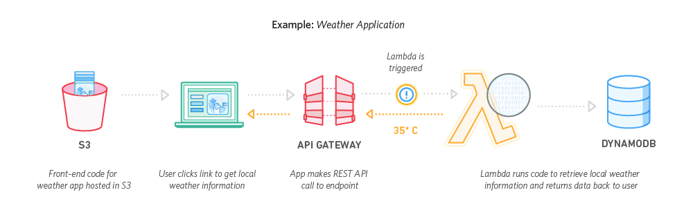
The advantage of these services is that instead of paying a fixed monthly fee for renting a compute instance in a datacenter (typically between $5 and $50 per month), you can "pay-as-you-go" based on the number of function calls that your application receives.
These services are priced by the number of function call requests per month -
| AWS Lambda | Google Cloud Functions | Azure Functions | |
|---|---|---|---|
| Free Requests Per Month | 1 million | 2 million | 1 million |
| Price Per Million Requests | $0.20 | $0.40 | $0.20 |
Each service also charges for the precise amount of CPU time used (rounded up to the nearest 100ms), but this pricing is a bit more complicated, so I'll just refer you their respective pricing pages.
The quickest way to get started is to use the open-source Serverless Framework, which provides an easy way to deploy Node.js, Python, Java, and Scala functions on either of the three services.
Serverless architecture has a lot of buzz right now, but I cannot personally vouch for how well it works in a production environment, so caveat emptor.
9. Use Docker to host multiple low-traffic apps on a single machine
Sometimes you might have multiple backend applications to run, but each without a very demanding CPU or memory footprint. In this situation, it can be an advantageous cost-cutting move to run all of the applications on the same machine instead of running each on a separate instance. This can be difficult, however, if the projects have differing dependencies (say, one requires Node v6.9 and another requires Node v8.4), or need to be run on different operating system distributions.

Docker is a containerization engine that provides an elegant solution to these issues. To make an application work with Docker, you can write a Dockerfile to include with the source code, specifying the base operating system and providing instructions to set up the project and dependencies. The resulting Docker container can be run on any operating system, making it very easy to consistently manage development/production environments and to avoid conflicting dependencies.
Docker-Compose is a tool that allows you write a configuration file to run multiple Docker containers at once. This makes it easy to run multiple lightweight applications, services, and database containers, all on the same system without needing to worry about conflicts.
Ports inside each container can be forwarded to ports on the host machine, so a simple reverse-proxy configuration (Nginx is a dependable, well-tested option) is all that is required to mount each application port behind a specific subdomain or URL route in order to make them all accessible via HTTPS on the host machine.
I have personally used this setup for a few of my personal projects in the past (and the present); it can save a lot of time and money if you are willing to take the time to get familiar the tools (which can, admittedly, have a steep learning curve at first).
10. Use Cloudflare for DNS management and SSL
Once you have your website/server hosted, you'll need a way to point your domain name to your content and to serve your domain over HTTPS.

Cloudflare is a domain management service backed by the likes of Google and Microsoft. At its core, Cloudflare allows you to point your domain name (and subdomains) to your website server(s). Beyond this basic functionality, however, it offers lots of free features that are hugely beneficial for anyone hosting a web app or API.
Benefit 1 - Security
Cloudflare will automatically protect your website from malicious traffic. Their massive infrastructure provides protection from DDoS (Distributed Denial of Service) attacks, and their firewall will protect your site from a continuously updated list of threats that are detected throughout their network.
Benefit 2 - Speed
Cloudflare will distribute your content quickly by sending it through a global CDN (content delivery network). The benefit of a CDN is that when someone visits the site, the data will be sent to them from a data center in their geographic region instead of from halfway around the world, allowing the page to load quicker.
Benefit 3 - Data Transfer Cost Savings
An added benefit to using a CDN is that by sending the cached content from Cloudflare's servers, you can reduce the bandwidth (and therefore the costs) from wherever your website is being hosted from. Cloudflare offers unlimited free bandwidth through their CDN.
Benefit 4 - Free SSL
Best of all, Cloudflare provides a free SSL certificate and automatically serves your website over HTTPS. This is very important for security (seriously, don't deploy a website without HTTPS), and would usually require server-side technical setup and annual fees; I've never seen another company (besides Let's Encrypt) offer it for free.
Cloudflare offers a somewhat absurd free plan, with which you can apply all of these benefits to any number of domain names.
A note on domain names - I don't know of any way to score a free domain name, so you might have to pay a registration fee and an annual fee. It's usually around $10/year, but you can get the first year for $1 or even for free if you shop around for deals. As an alternative, services like Heroku and GitHub can host your site behind their own custom subdomains for free, but you'll lose some brand flexibility with this option. I recommend buying a single domain (such as patricktriest.com) and deploying your apps for free on subdomains (such as blog.patricktriest.com) using Cloudflare.
Want more free stuff?
In my workflow, I also use Github to store source code and CircleCI to automate my application build/test/deployment processes. Both are completely free, of course, until you need more advanced, enterprise friendly capabilities.

If you need some beautiful free images check out Pexels and Unsplash, and for great icons, I would recommend Font Awesome and The Noun Project.
2017 is a great year to deploy a web app. If your app is a huge success, you can expect the costs to go up proportionally with the amount of traffic it receives, but with a well-optimized codebase and a scalable deployment setup, these costs can still be bounded within a very manageable range.
I hope that this post has been useful! Feel free to comment below with any other techniques and tactics for obtaining cheap web application hosting.

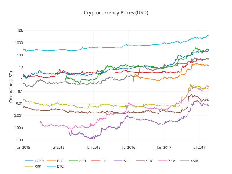
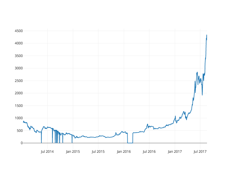


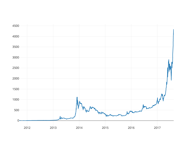
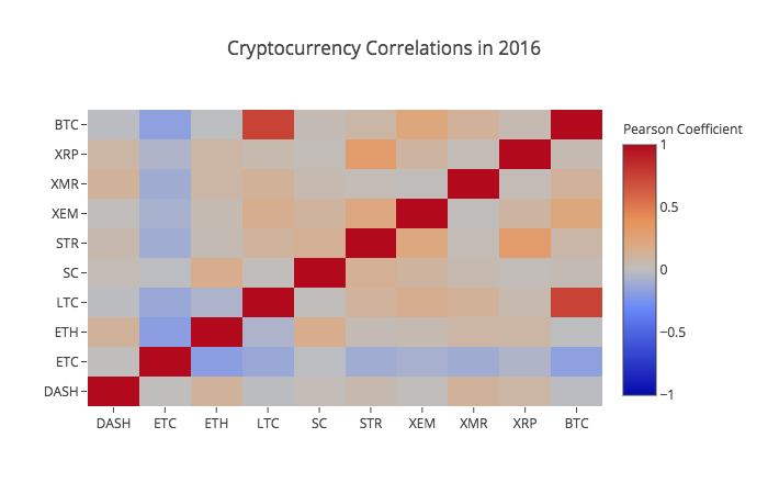
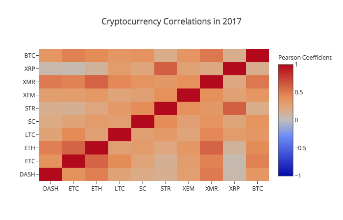


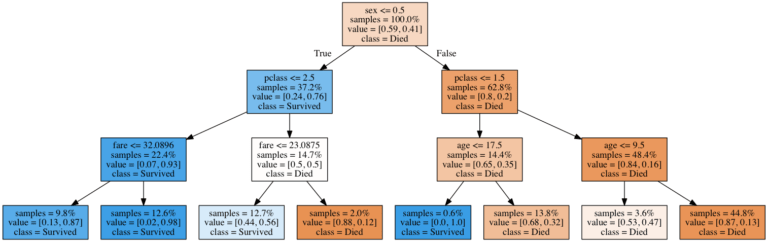
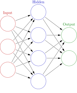
 From left to right: Hudson (30), Bess (25), Trevor (11 months), and Loraine Allison (2).
 John Jacob Astor IV
 Olaus Jorgensen Abelseth
 Autorickshaws at the Saket Metro Station
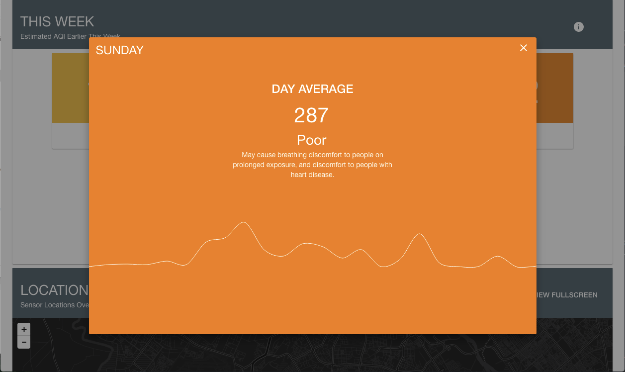 SocialCops Delhi Air Pollution Dashboard
 The prototype hardware, mid-assembly
 Autorickshaws at the Saket Metro station.
 One of the devices after being deployed for a week.
 The SocialCops team preparing the first device for deployment.
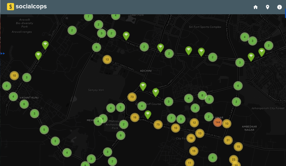

 Relay Wiring.
 Relay Wiring.